Applied Linear Algebra - Packet 04

Packet 04

Tutorial: Theory of Matrices in 2D and 3D

Matrix multiplication

Suppose we have a matrix $A$ and a vector $u$ that $A$ acts upon. We have written “$Au$” for the output vector given by letting $A$ act on $u$.

Matrices act by sending vectors to other vectors. It is useful to consider another matrix that acts upon the output vector. For example, if $𝐯:=A𝐮$, and if $B$ is a matrix that acts upon $v$, we can write $B(A𝐮)=B𝐯$. (The colon in $𝐯:=A𝐮$ means “$𝐯$ is defined as $A𝐮$.”)

Suppose we define $𝐰:=B𝐯$, so that $𝐰=B(A𝐮)$. Then we say that $w$ is the output of $𝐮$ under a composition of actions of the matrices $A$ and $B$. It turns out that if we start with two matrices $A$ and $B$, the composition action (letting the matrices act consecutively) can itself be represented by a single matrix. (The composition of linear transformations is a linear transformation.) Let us find this matrix in the case when $A$ and $B$ are $2\times 2$ matrices.

Suppose the entries of $A$ and $B$ are given by

$$A=\left(\begin{array}{cc}{a}_{11}& a_{12}\\ a_{21}& a_{22}\end{array}\right),B=\left(\begin{array}{cc}{b}_{11}& b_{12}\\ b_{21}& b_{22}\end{array}\right).$$

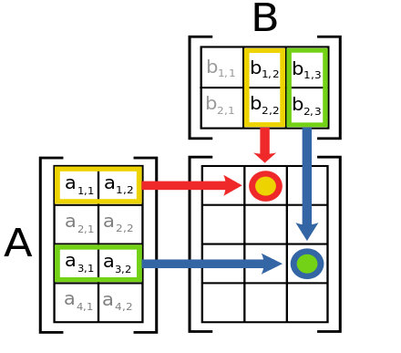
Now compute the action of $A$ followed by the action of $B$ on the vector $𝐮=\left(\begin{array}{c}{u}_1\\ u_2\end{array}\right)$:

$$\begin{array}{cc}B(A𝐮)& =\left(\begin{array}{cc}{b}_{11}& b_{12}\\ b_{21}& b_{22}\end{array}\right)\left(\left(\begin{array}{cc}{a}_{11}& a_{12}\\ a_{21}& a_{22}\end{array}\right)\left(\begin{array}{c}{u}_1\\ u_2\end{array}\right)\right)\\ & =\left(\begin{array}{cc}{b}_{11}& b_{12}\\ b_{21}& b_{22}\end{array}\right)\left(\begin{array}{c}{a}_{11}{u}_1+a_{12}{u}_2\\ a_{21}{u}_1+a_{22}{u}_2\end{array}\right)\\ & =\left(\begin{array}{c}{b}_{11}(a_{11}{u}_1+a_{12}{u}_2)+b_{12}(a_{21}{u}_1+a_{22}{u}_2)\\ b_{21}(a_{11}{u}_1+a_{12}{u}_2)+b_{22}(a_{21}{u}_1+a_{22}{u}_2)\end{array}\right)\\ & =\left(\begin{array}{c}(b_{11}{a}_{11}+b_{12}{a}_{21})u_1+(b_{11}{a}_{12}+b_{12}{a}_{22})u_2\\ (b_{21}{a}_{11}+b_{22}{a}_{21})u_1+(b_{21}{a}_{12}+b_{22}{a}_{22})u_2\end{array}\right)\\ & =\left(\begin{array}{cc}{b}_{11}{a}_{11}+b_{12}{a}_{21}& b_{11}{a}_{12}+b_{12}{a}_{22}\\ b_{21}{a}_{11}+b_{22}{a}_{21}& b_{21}{a}_{12}+b_{22}{a}_{22}\end{array}\right)\left(\begin{array}{c}{u}_1\\ u_2\end{array}\right).\end{array}$$

Therefore, we define the product matrix $BA$ by this formula:

$$BA=\left(\begin{array}{cc}{b}_{11}& b_{12}\\ b_{21}& b_{22}\end{array}\right)\left(\begin{array}{cc}{a}_{11}& a_{12}\\ a_{21}& a_{22}\end{array}\right)=\left(\begin{array}{cc}{b}_{11}{a}_{11}+b_{12}{a}_{21}& b_{11}{a}_{12}+b_{12}{a}_{22}\\ b_{21}{a}_{11}+b_{22}{a}_{21}& b_{21}{a}_{12}+b_{22}{a}_{22}\end{array}\right).$$

With this definition and the above reasoning, we have that $B(A𝐮)=(BA)𝐮$. (Because of this equality, we can omit the parentheses and write simply $BA𝐮$, since the result is the same whether you act first by $A$ and then by $B$ or instead you first multiply the matrices and then act by $BA$.)

Just as for the formula for a matrix acting on a vector, we have multiple ways to interpret the formula for the matrix $BA$.

• Each entry of the product matrix $BA$ is given by taking the dot product of a row of $B$ with a column of $A$.
• Each column of the product matrix $BA$ is given by letting $B$ act upon the corresponding column vector of $A$. In other words, $BA=\left(\begin{array}{cc}B{𝐚}_1& B{𝐚}_2\end{array}\right)$. (Recall that the action of $B$ upon ${𝐚}_i$ has two interpretations of its own!)
• Each row of the product matrix $BA$ is given by letting the entries in the corresponding row vector of $B$ provide the coefficients for a linear combination of the rows of $A$. The first of these interpretations is best for doing calculations, and the second is best for understanding abstract theory.

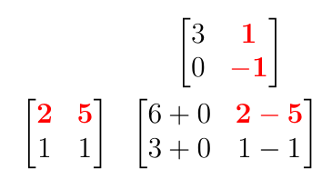
Bottom-Right Method for computing $AB$: E.g.:

Max Born, Nobel Prize lecture:

Question 04-01

Some matrix products

Compute the following matrix products by hand:

• (a) $\left(\begin{array}{cc}2& 3\\ 1& -5\end{array}\right)\left(\begin{array}{ccc}4& 3& 6\\ 1& -2& 3\end{array}\right)$
• (b) $\left(\begin{array}{ccc}1& 3& -5\\ 0& -2& 1\\ 0& 0& 4\end{array}\right)\left(\begin{array}{ccc}2& 1& 1\\ 0& -1& 3\\ 0& 0& 2\end{array}\right)$

In both (a) and (b) there are three matrices: two are given and their product is the third. In (a), what size vectors do these three matrices act upon? (How many components?) In (b), what do you notice about the nature of the two matrices and their resulting product? Can you guess a rule that generalizes this fact?

Question 04-02

Double rotation

Show that ${\left(\begin{array}{cc}\cos \theta & -\sin \theta \\ \sin \theta & \cos \theta \end{array}\right)}^2=\left(\begin{array}{cc}\cos (2\theta )& -\sin (2\theta )\\ \sin (2\theta )& \cos (2\theta )\end{array}\right)$, in other words two rotations by $\theta$ is equivalent to one rotation by $2\theta$.

Exercise 04-01

Nilpotent matrix

Define the matrix $A_{\lambda }$:

$$A_{\lambda }=\left(\begin{array}{ccccc}0& \lambda & 0& 0& 0\\ 0& 0& \lambda & 0& 0\\ 0& 0& 0& \lambda & 0\\ 0& 0& 0& 0& \lambda \\ 0& 0& 0& 0& 0\end{array}\right).$$

For $\lambda =2$, calculate the powers $A_2$, $A_2^2$, $A_2^3$, $A_2^4$, $A_2^5$.

(What special property does $A_{\lambda }$ have? A matrix with that property is said to be nilpotent.)

Identity matrix Notice that the diagonal matrix with $1$’s on the diagonal acts upon another vector or matrix by doing nothing:

$$\left(\begin{array}{ccc}1& 0& 0\\ 0& 1& 0\\ 0& 0& 1\end{array}\right)\left(\begin{array}{ccc}{a}_{11}& a_{12}& a_{13}\\ a_{21}& a_{22}& a_{23}\\ a_{31}& a_{32}& a_{33}\end{array}\right)=\left(\begin{array}{ccc}{a}_{11}& a_{12}& a_{13}\\ a_{21}& a_{22}& a_{23}\\ a_{31}& a_{32}& a_{33}\end{array}\right).$$

This matrix is called the identity matrix, since it preserves the identity of whatever it acts upon. It is frequently written “$I$”, regardless of the size of the matrix. So $I𝐮=𝐮$ for any $𝐮$.

Sometimes $I$ is written more specifically as $I_n$, where $n$ is the number of rows or columns. (Identity matrices always have the same number of rows and columns.)

Exercise 04-02

Reflections square to identity

Show that ${\left[{\mathrm{refl}}_{𝐯}\right]}^2=I_2$ for any $𝐯=\left(\begin{array}{c}{v}_1\\ v_2\end{array}\right)$ with $𝐯\cdot 𝐯=1$.

This means that reflecting twice across the same line gives back the original vector. (In 2D the hyperplane of reflection is just a line.)

Matrices acting on matrices

It is useful to think of matrices as acting upon other matrices by multiplying on the left. The effect is the same as the effect of acting on a vector, but it performs this (same) action on each column vector separately. The action is therefore the same across any given row.

Diagonal matrices When two diagonal matrices are multiplied, the result is a diagonal matrix. The diagonal entries of the product are simply the products of the diagonal entries:

$$\left(\begin{array}{ccc}{a}_1& 0& 0\\ 0& a_2& 0\\ 0& 0& a_3\end{array}\right)\left(\begin{array}{ccc}{b}_1& 0& 0\\ 0& b_2& 0\\ 0& 0& b_3\end{array}\right)=\left(\begin{array}{ccc}{a}_1{b}_1& 0& 0\\ 0& a_2{b}_2& 0\\ 0& 0& a_3{b}_3\end{array}\right).$$

A consequence is that diagonal matrices commute with each other: $AB=BA$ when $A,B$ are both diagonal. (As seen with 3D rotations, frequently this is not true for matrix multiplication.)

Row-scale matrices The diagonal matrices

$$A_1(\lambda )=\left(\begin{array}{ccc}\lambda & 0& 0\\ 0& 1& 0\\ 0& 0& 1\end{array}\right),A_2(\lambda )=\left(\begin{array}{ccc}1& 0& 0\\ 0& \lambda & 0\\ 0& 0& 1\end{array}\right),A_3(\lambda )=\left(\begin{array}{ccc}1& 0& 0\\ 0& 1& 0\\ 0& 0& \lambda \end{array}\right)$$

have the effect of scaling rows $\mathrm{1,2,3}$ (respectively) by the number $\lambda$, without changing other rows, when they are multiplied on a vector or a matrix on the left. These matrices are called row-scale matrices.

Permutation matrices When two permutation matrices are multiplied, the result is a permutation matrix. For example:

$$\left(\begin{array}{ccc}0& 1& 0\\ 1& 0& 0\\ 0& 0& 1\end{array}\right)\left(\begin{array}{ccc}1& 0& 0\\ 0& 0& 1\\ 0& 1& 0\end{array}\right)=\left(\begin{array}{ccc}0& 0& 1\\ 1& 0& 0\\ 0& 1& 0\end{array}\right).$$

Question 04-03

Permutation matrices

Explain why the product of two permutation matrices is always a permutation matrix. (Recall the definition: a matrix is a permutation matrix when each row and each column contains exactly one $1$ and the other entries are $0$.)

Row-swap matrices A permutation matrix acts upon another matrix (multiplying on the left) by permuting the rows of the matrix, in the same way that it would permute the rows of a vector:

$$\left(\begin{array}{cc}0& 1\\ 1& 0\end{array}\right)\left(\begin{array}{cc}{a}_{11}& a_{12}\\ a_{21}& a_{22}\end{array}\right)=\left(\begin{array}{cc}{a}_{21}& a_{22}\\ a_{11}& a_{12}\end{array}\right).$$

The most important permutation type is one which simply swaps two rows and leaves the others unchanged. This type of matrix is called a row-swap matrix.

The row-swap action is performed by a permutation matrix which has $1$’s on the diagonal except for two rows. In these two rows, the ones from a diagonal matrix are swapped with each other.

Example

Row-swap example

The $4\times 4$ matrix which swaps rows $2$ and $4$ (of a vector or another matrix) works like this:

$$\left(\begin{array}{cccc}1& 0& 0& 0\\ 0& 0& 0& 1\\ 0& 0& 1& 0\\ 0& 1& 0& 0\end{array}\right)\left(\begin{array}{cccc}{a}_{11}& a_{12}& a_{13}& a_{14}\\ a_{21}& a_{22}& a_{23}& a_{24}\\ a_{31}& a_{32}& a_{33}& a_{34}\\ a_{41}& a_{42}& a_{43}& a_{44}\end{array}\right)=\left(\begin{array}{cccc}{a}_{11}& a_{12}& a_{13}& a_{14}\\ a_{41}& a_{42}& a_{43}& a_{44}\\ a_{31}& a_{32}& a_{33}& a_{34}\\ a_{21}& a_{22}& a_{23}& a_{24}\end{array}\right).$$

To obtain this row-swap matrix, start with the diagonal matrix with $1$’s along the diagonal, and then swap rows $2$ and $4$.

Row-add matrices A matrix that has $1$’s on the diagonal and the other entries $0$’s, except for a single additional entry $\lambda$, is called an elementary shear matrix, or a row-add matrix:

$$\left(\begin{array}{ccc}1& \lambda & 0\\ 0& 1& 0\\ 0& 0& 1\end{array}\right),\left(\begin{array}{ccc}1& 0& 0\\ 0& 1& 0\\ \lambda & 0& 1\end{array}\right),\text{etc.}$$

If the $\lambda$ entry is in the $i^{th}$ row and $j^{th}$ column, this matrix acts by taking the $j^{th}$ row (of a matrix or vector that it’s acting upon) and adding it into the $i^{th}$ row with a $\lambda$ coefficient:

$$\left(\begin{array}{ccc}1& \lambda & 0\\ 0& 1& 0\\ 0& 0& 1\end{array}\right)\left(\begin{array}{ccc}{a}_{11}& a_{12}& a_{13}\\ a_{21}& a_{22}& a_{23}\\ a_{31}& a_{32}& a_{33}\end{array}\right)=\left(\begin{array}{ccc}{a}_{11}+\lambda a_{21}& a_{12}+\lambda a_{22}& a_{13}+\lambda a_{23}\\ a_{21}& a_{22}& a_{23}\\ a_{31}& a_{32}& a_{33}\end{array}\right).$$

Remember that when a matrix is multiplied on the left on a vector or a matrix, the top row of the matrix controls the top row of the output.

Matrix algebra

Matrix addition and scaling Matrices can be added, subtracted, and multiplied by scalers, just like vectors. These operations are done componentwise:

$$\begin{array}{cc}\left(\begin{array}{cc}{a}_{11}& a_{12}\\ a_{21}& a_{22}\end{array}\right)+\left(\begin{array}{cc}{b}_{11}& b_{12}\\ b_{21}& b_{22}\end{array}\right)& =\left(\begin{array}{cc}{a}_{11}+b_{11}& a_{12}+b_{12}\\ a_{21}+b_{21}& a_{22}+b_{22}\end{array}\right),\\ \lambda \left(\begin{array}{cc}{a}_{11}& a_{12}\\ a_{21}& a_{22}\end{array}\right)& =\left(\begin{array}{cc}\lambda a_{11}& \lambda a_{12}\\ \lambda a_{21}& \lambda a_{22}\end{array}\right).\end{array}$$

In terms of the actions performed by these matrices, addition is like addition of functions: the action of a sum of matrices is to give the sum of the outputs under the actions of the separate matrices. For functions, this would be written $(f+g)(x)=f(x)+g(x)$. For matrices, we write $(A+B)𝐮=A𝐮+B𝐮$, and similarly for subtraction, scalar multiples, and other variations on basic algebra operations.

Matrix distributivity It is important to notice that matrix multiplication is compatible with matrix addition in the usual sense of distributivity:

$$A(B+C)=AB+AC.$$

One way to prove this formula is to show that it is true after both sides are applied to an arbitrary vector $𝐮$. (To complete the proof, let $𝐮$ take the specific value of each standard basis vector ${𝐞}_i$ in turn, and you find that column $i$ of the matrices on each side must agree.) To show the equality after multiplying both sides on an arbitrary $𝐮$, we need to check distributivity of matrix actions on vectors in general:

Question 04-04

Linearity / Distributivity of matrix actions

Show that $A(𝐮+𝐯)=A𝐮+A𝐯$ whenever a matrix $A$ acts on vectors $𝐮$ and $𝐯$.

Hint: first try this with a $3\times 3$ matrix and 3D vector with arbitrary entries. Then to show it in general, use the “summation notation” for the matrix action on a vector:

$${(A𝐮)}_i=\sum _{j=1}^n{a}_{ij}{u}_j.$$

Matrix division For real numbers, division and multiplication are inverse processes, meaning that division “undoes” the action of multiplication, and vice versa.

Any number can divide another number provided it is not zero. For matrices, the situation is more complex, because “being zero” is more complex. Many matrices have non-zero entries, yet they “act as zero” upon certain other vectors. When this happens, the action cannot be “undone”, because you cannot divide by the zero action performed on those vectors.

Example

Projection is not invertible

Consider the projection matrix $\left(\begin{array}{cc}1& 0\\ 0& 0\end{array}\right)$ which sends a vector $(x,y)$ to the vector $(x,0)$. This matrix acts by zero upon any vector $(0,y)$, sending $(0,y)$ to $(\mathrm{0,0})$. This action cannot be undone! (What specific vector would the inverse action send $(\mathrm{0,0})$ to?)

So, some matrices can be divisors. These are called invertible matrices. Others cannot, and these are called non-invertible matrices. A matrix $A$ is invertible when the inverse matrix $A^{-1}$ exists.

When it exists, an inverse matrix $A^{-1}$ acts by undoing multiplication by $A$. Concretely, this means:

$$A^{-1}A𝐮=𝐮,A{A}^{-1}𝐮=𝐮\text{for any vector }𝐮.$$

Notice in the second formula that the action of $A$ can be undone before $A$ even acts. (Ordinary division also works like this!) Another way to look at it is that $A$ acts by undoing the effect of $A^{-1}$. (Ordinary division: multiplication by $5$ undoes the effect of multiplying by $1/5$.)

Recall the “identity matrix” $I$ which satisfies $I𝐮=𝐮$ for any $𝐮$. So we can write the above formula using matrices:

$$A^{-1}A=I,A{A}^{-1}=I.$$

Notice that we have to write both formulas because matrix multiplication is not commutative! (Ordinary division: $5\cdot (1/5)=1$ and $(1/5)\cdot 5=1$ are equivalent because $ab=ba$ for any numbers.)

Inverse of $2\times 2$ matrices There is a general formula for the inverse of any $2\times 2$ matrix that should be memorized:

$$A=\left(\begin{array}{cc}a& b\\ c& d\end{array}\right),A^{-1}=\frac{1}{ad-bc}\left(\begin{array}{cc}d& -b\\ -c& a\end{array}\right).$$

Exercise 04-03

Checking formula for $2\times 2$ inverse

Check the formula for $A^{-1}$ for a $2\times 2$ matrix $A$ by computing by hand $A{A}^{-1}$ and $A^{-1}A$. (You should obtain $\left(\begin{array}{cc}1& 0\\ 0& 1\end{array}\right)$ in both cases.)

Which $2\times 2$ matrices $A$ have an inverse?

(Hint: you just checked a formula that works whenever it makes sense, so there is an inverse whenever it makes sense, given by the formula. Suppose $a,b,c,d$ are such that the formula does not make sense. Can you find a vector $𝐮\ne \mathrm{𝟎}$ which is sent to $\mathrm{𝟎}$ by $A$?)

Exercise 04-04

Inverse of a reflection

Show (in 2D) that the matrix of a reflection is the inverse of itself. Show this first abstractly (using the definition of inverse), and then concretely (using the formulas for reflection and inverse matrices).

Exercise 04-05

Inverse of a rotation

Show (in 2D) that the inverse of the matrix of rotation by $\theta$ is the matrix of rotation by $-\theta$.

The inverse of $A$ is useful for finding a vector $𝐮$ which is sent to a given vector $𝐯$ by the action of a given matrix $A$:

$$A𝐮=𝐯\text{if and only if}𝐮=A^{-1}𝐯.$$

If we know $A$ and $𝐯$, and we want $𝐮$, this method will give us $𝐮$.

Example

Inverse matrix to find preimage

Problem: Define

$$A=\left(\begin{array}{cc}1& 2\\ -2& -3\end{array}\right),𝐯=\left(\begin{array}{c}1\\ 4\end{array}\right).$$

Find a vector $𝐮$ with the property that $A𝐮=𝐯$, meaning that $A$ sends $𝐮$ to the given $𝐯$.

Solution: First we compute $A^{-1}$ using the formula. We have $ad-bc=-3--4=1$, so $A^{-1}=\left(\begin{array}{cc}-3& -2\\ 2& 1\end{array}\right)$. Now compute that $A^{-1}𝐯=\left(\begin{array}{c}-11\\ 6\end{array}\right)$, and this is our answer for $𝐮$. Check this answer by computing $A\left(\begin{array}{c}-11\\ 6\end{array}\right)=\left(\begin{array}{c}1\\ 4\end{array}\right)$, as expected.

Exercise 04-06

Inverse matrix to find preimage

Repeat the previous example for this data:

$$A=\left(\begin{array}{cc}1& -3\\ -2& 4\end{array}\right),𝐯=\left(\begin{array}{c}-4\\ 2\end{array}\right).$$

Determinant of $2\times 2$ matrices The determinant of a matrix $A$, written $\det A$, is a single number that is associated to the matrix.

For a $2\times 2$ matrix, the determinant is given by the formula in the divisor of the formula for $A^{-1}$:

$$\det A=ad-bc\text{when}A=\left(\begin{array}{cc}a& b\\ c& d\end{array}\right).$$

We will learn many things about determinants. The important thing for now is that $A^{-1}$ exists if and only if $\det A\ne 0$.

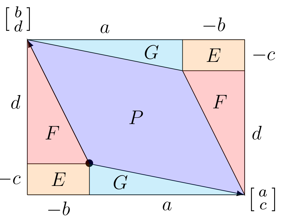
Optional: interpretation of $2\times 2$ determinant Just for fun, here is a visual proof (by S. Golomb) that $\det A$ gives the area of the parallelogram spanned by the column vectors of 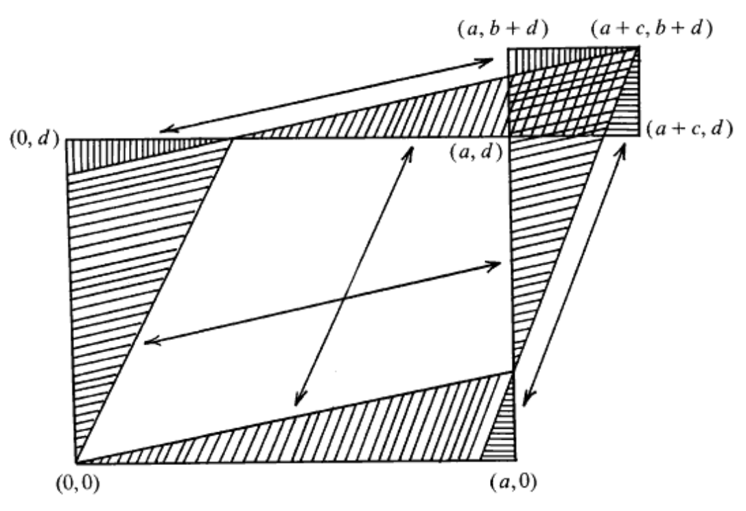$A$, namely $\left(\begin{array}{c}a\\ c\end{array}\right)$ and $\left(\begin{array}{c}b\\ d\end{array}\right)$: Here is another visual for parallelograms from obtuse vectors:

Eigenvectors, eigenvalues

We saw that standard basis vectors ${𝐞}_i$ are eigenvectors for diagonal matrices, and the diagonal entries are the eigenvalues. If $A$ has diagonal entries $a_1,a_2,a_3$, then $A{𝐞}_i=a_i{𝐞}_i$.

Now consider the problem of finding eigenvectors and eigenvalues for a non-diagonal matrix $A$. This means finding a vector $𝐯\ne \mathrm{𝟎}$ and a scalar $\lambda$ such that $A𝐯=\lambda 𝐯$.

Suppose we start with a hypothetical $\lambda$. Write $\lambda I_2$ for the matrix $\left(\begin{array}{cc}\lambda & 0\\ 0& \lambda \end{array}\right)$. So we wish to solve $A𝐯=(\lambda I_2)𝐯$, which is equivalent to $(A-\lambda I_2)𝐯=0$. Now write $A_{\lambda }:=A-\lambda I_2$. So we wish to find $𝐯$ such that $A_{\lambda }𝐯=\mathrm{𝟎}$.

Notice that if $A_{\lambda }$ is invertible, then there is no solution. (The only solution would be $𝐯=0$ and that is not allowed for an eigenvector.) The reason is that if $A_{\lambda }^{-1}$ exists, we can let it act upon both sides of the equation $A_{\lambda }𝐯=\mathrm{𝟎}$ to obtain $𝐯=A_{\lambda }^{-1}\mathrm{𝟎}=0$. Therefore, we only have a chance of solving this if $A_{\lambda }$ is non-invertible. Recall from above that $A_{\lambda }$ is non-invertible precisely when $\det A_{\lambda }=0$.

It turns out we can solve the equation if $\det A_{\lambda }=0$. Let us do this by hand for $2\times 2$ matrices.

Derivation that if $\det M=0$ then $M𝐯=\mathrm{𝟎}$ can be solved with $𝐯\ne 0$

Let $M=\left(\begin{array}{cc}a& b\\ c& d\end{array}\right)$. Assume $\det M=0$, which means $ad-bc=0$ or $ad=bc$ or $c/a=d/b$. Write $x$ for the common ratio $c/a=d/b$. Thus $M=\left(\begin{array}{cc}a& b\\ xa& xb\end{array}\right)$, and now we wish to solve the equation:

$$\left(\begin{array}{cc}a& b\\ xa& xb\end{array}\right)\left(\begin{array}{c}{v}_1\\ v_2\end{array}\right)=\left(\begin{array}{c}0\\ 0\end{array}\right).$$

This means $a{v}_1+b{v}_2=0$ and $xa{v}_1+xb{v}_2=0$. Dividing the latter by $x$ we arrive at the former, so we can take any $(v_1,v_2)$ that satisfy $v_1/v_2=-b/a$. Let us choose $(v_1,v_2)=(-b,a)$. You can now check directly that it works:

$$\left(\begin{array}{cc}a& b\\ xa& xb\end{array}\right)\left(\begin{array}{c}-b\\ a\end{array}\right)=\left(\begin{array}{c}0\\ 0\end{array}\right).$$

If $\det A_{\lambda }=0$, there must be a vector $𝐯\ne \mathrm{𝟎}$ such that $A𝐯=\lambda 𝐯$ for some scalar $\lambda$

Proof: Define $A=\left(\begin{array}{cc}a& b\\ c& d\end{array}\right)$, and so

$$A_{\lambda }=\left(\begin{array}{cc}a& b\\ c& d\end{array}\right)-\left(\begin{array}{cc}\lambda & 0\\ 0& \lambda \end{array}\right)=\left(\begin{array}{cc}a-\lambda & b\\ c& d-\lambda \end{array}\right).$$

Suppose $\det A_{\lambda }=0$. By the formula for $\det$, this means $(a-\lambda )(d-\lambda )-bc=0$. That is a quadratic equation in $\lambda$ and could be rewritten as ${\lambda }^2+(-a-d)\lambda +(ad-bc)=0$. By the quadratic formula, the solutions are $\lambda =\frac{1}{2}(a+d\pm \sqrt{{(a-d)}^2+4bc})$. Write these two solutions as ${\lambda }_1$ and ${\lambda }_2$.

So we have found ${\lambda }_1$ and ${\lambda }_2$ with $\det A_{{\lambda }_1}=0$ and $\det A_{{\lambda }_2}=0$. In either case we can solve for a ${𝐯}_1\ne \mathrm{𝟎}$ such that $A_{{\lambda }_1}{𝐯}_1=0$ and a ${𝐯}_2$ such that $A_{{\lambda }_1}{𝐯}_2=0$ using the method in the box above.

Example

Finding eigenvectors and eigenvalues

Problem: Define $A=\left(\begin{array}{cc}1& 6\\ 5& 2\end{array}\right)$. Find the two eigenvalues and some (any) two corresponding eigenvectors of $A$.

Solution: First write $A_{\lambda }=\left(\begin{array}{cc}1-\lambda & 6\\ 5& 2-\lambda \end{array}\right)$. Then $\det A_{\lambda }=0$ means $(1-\lambda )(2-\lambda )-30=0$. Solve this quadratic equation to obtain ${\lambda }_1=7$ and ${\lambda }_2=-4$. We have found the two eigenvalues.

Next, write out the matrices

$$A_{{\lambda }_1}=\left(\begin{array}{cc}-6& 6\\ 5& -5\end{array}\right),A_{{\lambda }_2}=\left(\begin{array}{cc}5& 6\\ 5& 6\end{array}\right).$$

Our goal is to find ${𝐯}_1$ and ${𝐯}_2$ such that $A_{{\lambda }_i}{𝐯}_i=0$. We can guess two solutions: let ${𝐯}_1=\left(\begin{array}{c}1\\ 1\end{array}\right)$ and let ${𝐯}_2=\left(\begin{array}{c}-6\\ 5\end{array}\right)$. To check that these are indeed eigenvectors of the original $A$ corresponding to ${\lambda }_1=7$ and ${\lambda }_2=-4$, compute:

$$\left(\begin{array}{cc}1& 6\\ 5& 2\end{array}\right)\left(\begin{array}{c}1\\ 1\end{array}\right)=\left(\begin{array}{c}7\\ 7\end{array}\right)=7\left(\begin{array}{c}1\\ 1\end{array}\right),\left(\begin{array}{cc}1& 6\\ 5& 2\end{array}\right)\left(\begin{array}{c}-6\\ 5\end{array}\right)=\left(\begin{array}{c}24\\ -20\end{array}\right)=-4\left(\begin{array}{c}-6\\ 5\end{array}\right).$$

You could also use the procedure in the gray box “Derivation.” For $A_{{\lambda }_1}$ we have $x=-5/6$, and for $A_{{\lambda }_2}$ we have $x=1$. Then we would get ${𝐯}_1=\left(\begin{array}{c}-6\\ -6\end{array}\right)$ and ${𝐯}_2=\left(\begin{array}{c}-6\\ 5\end{array}\right)$. Notice that the first eigenvector is a scalar multiple of ours above: $\left(\begin{array}{c}-6\\ -6\end{array}\right)=-6\left(\begin{array}{c}1\\ 1\end{array}\right)$.

This is true in general: if $A𝐯=\lambda 𝐯$, then $A(x𝐯)=\lambda (x𝐯)$. In other words, you can scale an eigenvector and the result is still an eigenvector with the same eigenvalue. This is because $Ax=xA$ when $x$ is a scalar, and of course $x\lambda =\lambda x$ when both are scalars. In yet other words, the line $⟨𝐯⟩$ spanned by an eigenvector $𝐯$, called an eigenline, is preserved by the matrix: every vector on this line is mapped back to something on this line.

Summary

• Matrices can be multiplied by each other. Express $A=\left(\begin{array}{ccc}{𝐚}_1& {𝐚}_2& {𝐚}_3\end{array}\right)$ as a row of column vectors; then $BA$ is the matrix which is the row of column vectors $\left(\begin{array}{ccc}B{𝐚}_1& B{𝐚}_2& B{𝐚}_3\end{array}\right)$. In other words, $BA$ is computed by letting $B$ act upon the columns of $A$.
• Matrices acting on vectors satisfy $A(𝐮+𝐯)=A𝐮+A𝐯$, and acting on matrices they satisfy $A(B+C)=AB+AC$.
• The identity matrix $I_3=\left(\begin{array}{ccc}1& 0& 0\\ 0& 1& 0\\ 0& 0& 1\end{array}\right)$ has the property that $I_{3}A=A$ and $A{I}_3=A$ for any other matrix $A$.
• Row-scale matrices act on a matrix (or vector) by scaling a chosen row. Row-swap matrices act by swapping two rows. Row-add matrices act by adding one row into another.
• An “invertible” matrix $A$ is one having an inverse $A^{-1}$, which has the property that $A^{-1}A=A{A}^{-1}=I_n$. (Here $A$ is an $n\times n$ matrix.) For a $2\times 2$ matrix, its inverse is given by a formula: $$$$

A=\begin{pmatrix} a&b\c&d \end{pmatrix},\quad A^{-1}=\frac{1}{ad-bc}\begin{pmatrix} d&-b\-c&a \end{pmatrix}.

- The inverse matrix $A^{-1}$ can be *used to solve for $\mathbf{u}$* in the equation $A\mathbf{u}=\mathbf{v}$, where $A$ and $\mathbf{v}$ are both given and $\mathbf{u}$ is sought. - The *determinant* $\det A$ for the $2\times 2$ matrix $A$ (as above) is the number $ad-bc$. The matrix $A$ is *invertible if and only if $\det A\neq 0$*. - Given the matrix $A$, an *eigenvector* $\mathbf{v}$ is a vector ($\neq 0$) such that *$A\mathbf{v}=\lambda\mathbf{v}$* for some scalar $\lambda$ called the *eigenvalue* corresponding to $\mathbf{v}$. - We can *find eigenvalues and eigenvectors* by: setting $\det(A-\lambda I_2)=0$ and solving a quadratic equation to find $\lambda_1$, $\lambda_2$, then plugging these in for $\lambda$ and writing $A_{\lambda_1}=A-\lambda_1 I_2$ and $A_{\lambda_1}=A-\lambda_1 I_2$, and then manually solving for vectors $\mathbf{v}_1$ and $\mathbf{v}_2$ satisfying $A_{\lambda_1}\mathbf{v}_1=0$ and $A_{\lambda_2}\mathbf{v}_2=0$. This is possible using the fact that one row of $A_{\lambda_i}$ will be a multiple $x$ times the other row. ## Problems due 14 Feb 2024 by 12:00pm ##### Problem 04-01 > [!question] Basic multiplications; differing sizes > > Define the following matrices: > $$ > A=\begin{pmatrix}1&2\\3&6\\2&1\end{pmatrix},\quad B=\begin{pmatrix}1&-1\\-1&0\end{pmatrix},\quad C=\begin{pmatrix}1&0&1\\1&3&3\end{pmatrix}. > $$ > Compute the matrix products: $AB$, $AC$, $(BC)A$, $B(CA)$. ##### Problem 04-02 > [!question] Row reduction using elementary matrices > > The row-scale, row-add, and row-swap matrices can be applied in a sequence to *manipulate the entries* of another matrix or vector. A very useful goal is to convert a matrix into an *upper-triangular* matrix, which is a matrix that has all entries *below* the main diagonal equal to zero. > > For example, the matrix $\begin{pmatrix}2&-4\\3&-1\end{pmatrix}$ can be manipulated into an upper-triangular matrix by adding $-3/2$ times row $1$ into row $2$, because $(-3/2)\cdot 2=-3$ and $-3+3=0$. This action is performed by the row-add matrix with $-3/2$ in the $2^{\text{nd}}$ row of the $1^{\text{st}}$ column: > $$ > \begin{pmatrix}1&0\\-3/2&1\end{pmatrix}\begin{pmatrix}2&-4\\3&-1\end{pmatrix}=\begin{pmatrix}2&-4\\0&5\end{pmatrix}. > $$ > Now, using a sequence of matrix actions chosen from the types *row-scale* and *row-add*, convert the matrix > $$ > A = \begin{pmatrix}3&2&-2\\15&12&-8\\9&2&-6\end{pmatrix} > $$ > into an upper-triangular matrix. (Hint: first create two zeros in the first column, then create the zero needed in the second column.) > > Now multiply together the manipulation matrices used to perform your actions (multiplied right-to-left in order of the actions so that the actions are composed). > > Finally, show that this product matrix converts the original matrix to an upper-triangular matrix by multiplying on the left. ##### Problem 04-03 > [!question] Matrix inversion to find preimages > > In each case below, show that $\det A\neq 0$, compute the inverse $A^{-1}$, and use it to find the vector $\mathbf{u}$ satisfying the equation: > - (a) $\begin{pmatrix}1&2\\3&5\end{pmatrix}\mathbf{u}=\begin{pmatrix}5\\-2\end{pmatrix}$ > - (b) $\begin{pmatrix}2&5\\-3&-7\end{pmatrix}\mathbf{u}=\begin{pmatrix}1\\8\end{pmatrix}$ ##### Problem 04-04 > [!question] Calculate eigenvalues and eigenvectors for $2\times 2$ matrix > > Imitate the Example to find the eigenvalues and eigenvectors for $A$: > $$ > A=\begin{pmatrix}7&4\\-3&-1\end{pmatrix}. > $$ ##### Problem 04-05 > [!question] Actions on the right: rows v. columns > > In this problem, we consider the action of a matrix upon another matrix by multiplication *on the right*. That is, the action of $B$ upon $A$ by sending $A$ to $AB$. (The effect is very similar to acting on the left, except that the roles of ‘rows’ and ‘columns’ are reversed!) > - (a) Describe the action of a $3\times 3$ matrix $B$ on the right upon a *row vector* $(v_1\;v_2\;v_3)$. (To obtain the formula, take the matrix product treating the row vector as a $1\times 3$ matrix. Now interpret the formula analogously to the first point in the Summary.) > - (b) Describe the action of $B$ multiplying on the right on a *matrix* $A$ in terms of the *row vectors* of $A$. > - (c) What does the matrix $B_3(\lambda)=\begin{pmatrix}1&0&0\\0&1&0\\0&0&\lambda\end{pmatrix}$ do to another $3\times 3$ matrix $A$ when it acts on the right? > - (d) What is the $3\times 3$ matrix that *swaps columns $i$ and $j$* by acting on the right? > - (e) What is the $3\times 3$ matrix that *adds column $j$ into column $i$* by acting on the right? ParseError: Can't use function '$' in math mode at position 22: …inverse matrix $̲A^{-1}$ can be …