Applied Linear Algebra - Packet 09

Packet 09

Matrices I: Reduction and Decomposition

A very important general method for understanding what matrices do when they act upon vectors is to transform them into matrices or products of matrices with standardized form. Each standardized form is designed to make certain aspects of matrix behavior very easy to see, or to make certain calculations that apply the matrix very easy to perform. Typically a matrix is converted to a standardized form using an algorithmic procedure that is run without intuitive or subjective assessment along the way, and the final result is studied afterwards.

In this packet we study a standardized form called ‘LU factorization’ that is produced using the technique of elimination. Given the LU factorization (or a refinement of part of it called row-echelon form or reduced row-echelon form), one can read off qualitative aspects of the matrix such as its rank, which is the dimension of its image subspace, as well as provide a basis for the image and a basis for the kernel, which is the subspace that is reduced to zero by the matrix action.

In addition to this qualitative information about the action of a matrix on some vectors, the LU factorization can be followed by another important technique called back-substitution. The combined process is typically used for inverting matrix equations such as these:

The vector inverse of under the action of is the vector which sends to . The matrix inverse of under the action of is the matrix which is sent to by the action of multiplying it on the left. (In the second case, if is the identity, then we are just computing .) We will see below how the factorization process followed by back-substitution allows us to find or .

LU factorization

An LU factorization of a matrix is simply a lower triangular matrix and an upper triangular matrix such that .

For example 1.

or 2.

Observe:

• In 1., both and have ones on the diagonal, and all matrices are square.
• In 2., and are not square, has ones on the diagonal, while has other values: .

We require the matrix to have ones on the diagonal, while the matrix may have other diagonal values.

A more general rule for called “row-echelon form” will be explained below; it is applicable when zeros on the diagonal crop up in the process; in essence it means the entries should be mashed “high and to the right.”

Keys to LU factorization

The principle of elimination is to use row-add matrices acting on the left in order to eliminate nonzero entries of that are below the main diagonal entries, clearing a column. These row-add matrices are then collected into a single lower-triangular matrix that combines the actions of all of them.

Creating columns: Observe first that we can combine row-add matrices which add from the same row into a single matrix having a single column of nonzero subdiagonal entries, for example:

The order in the product on the RHS does not matter!

Question 09-01

Order doesn’t matter when multiplying row-add matrices of the same column

Explain why (or prove algebraically that) order does not matter when multiplying row-add matrices with their nonzero subdiagonal entries lying in the same column. Explain this in general, not just for the matrix above.

Combining columns: Furthermore, we can break up any lower-triangular matrix into a product of single-column matrices like the one above:

Combining columns – order matters

The three factors in the RHS product cannot be reordered without changing the result!

By combining the above two factorizations, we can write any lower-triangular matrix (with ones on the diagonal) as a product of row-add matrices, and these row-add matrices can be grouped into single-column row-add combo matrices. If is lower-triangular with rows, and we write for the single-column combo with nonzeros in the column, then we have . When you see you should think “single-column, row-add combo” and remember that the column of nonzeros lies below the main diagonal of ones.

Inverse of : The last critical fact is that the inverse of any single-column row-add combo is the same matrix but with opposite signs on the subdiagonal entries:

Computing LU factorizations

Here is the plan:

1. Postulate hypothetically that , where are single-column row-add combos which combine to form the hypothetical . We know and we seek and .
2. Act upon and on the left simultaneously by , then by , etc., through . We must invent , etc. as we go along:
   1. Choose such that has all zeros in the first column on the subdiagonal: In each nonzero subdiagonal entry of , put such that row-add of the top entry into entry eliminates entry , and so on to create the entire first column of which acts to clear the first column of .
   2. Continue with chosen such that now has zeros in the first and second columns, and has subdiagonal entries in the second column.
   3. Continue through and obtain . By flipping signs on for , we now know and simply combine the subdiagonal columns of all to create the whole .
   4. Notice! The matrix is exactly the unique single-column row-add combo matrix which has column cleared by whatever clears the column of . In other words, we cook up so that the same elimination works both on and on , the difference being that has a at the top entry by definition, while the corresponding entry of may have other values.

In other words, we find the matrices by backwards reasoning: row-add eliminations performed on should simultaneously effect eliminations on , converting them each to the identity matrix . If this works, we know we have the ingredients inside the factorization .

Example

Basic LU factorization

Problem: Show how to obtain the LU factorization:

Solution: Full steps for the product multiplication showing as above can be found here. Full steps for the reverse, factoring into , can be found here. (Click “Details” to show the steps.) We explain the latter details below. You are encouraged to use MatrixCalc.org to help you master the process, but remember that on the exams you must be able to run the process by hand.

Since is a matrix, we are looking for such that and each is a single-column row-add combo matrix. Since the factorization is given to us, we know the answers should be:

Obtain these as follows. To eliminate the subdiagonal entries in the first column of , we must add times row into row , then times row into row , and then times row into row .

To cook up , we first place ones on the diagonal, zeros elsewhere (namely ). Then we arrange the first column so that it’s cleared by the same sequence of steps, except now we have in the first row whereas had . Thus: times added to gives , then times added to gives , and times added to gives . The sequence is therefore appropriate for the first column in , since it will be cleared by whatever row-adds clear the first column of .

We have thus found as the matrix which is sent to by the action of the elimination process just described. This elimination process is represented by the action of the single-column row-add combo matrix:

and therefore just given is the inverse of that we sought: since .

After applying the process to and finding , we proceed to find , creating its column in order to clear the from the second column of :

Therefore

is the right choice for , and we are almost finished. Observe that . Thus:

and so

Question 09-02

Compute LU factorization

Find the LU factorization of the matrix .

Exercise 09-01

Computing LU factorization

Find the LU factorization of .

Exercise 09-02

Computing LU factorization

Find the LU factorization of .

Exercise 09-03

Computing LU factorization

Find the LU factorization of .

Pivoting

The algorithm presented above for LU factorization can fail down because of zeros. For example, consider :

We cannot even begin to eliminate using row-add steps. In this situation, it is best to pivot to a different top row by using a row-swap permutation. The new top row is sometimes called the pivot row, and the new entry used to eliminate others by row-adding may be called the pivot entry or simply the pivot.

Write for the row-swap matrix that swaps rows and . After pivoting, we have a new matrix:

The new matrix has an LU factorization now:

It is appropriate to say that “ has an LU factorization with pivots”, or to say that “we have a factorization .” We do not say simply that “ has an LU factorization” if pivots are required.

Every matrix has a factorization of the form .

Numerical methods

For numerical stability, it is preferable to always pivot to the largest entry in a given column before performing elimination. This technique is called “partial pivoting.”

(“Complete pivoting” refers to a technique where elimination is performed to clear any uncleared column by choosing the largest remaining entry across the matrix. It is computationally expensive and therefore rarely used.)

The general procedure for computing factorizations is fairly complex because the natural algorithm interlaces elimination (using factors ) with permutations for the pivots (using row-swap matrices ). You are not required to master this procedure for exams.

The general process of computing by successive elimination of terms with pivots, clearing out one column at a time, is called row reduction (see below). You are required to master row-reduction for exams.

The difference between row-reduction and the procedure for is that in the latter we do not keep track of and and do not calculate and , we simply perform the row-add operations on until the factor inside is gone (by clearing columns) and the result is .

Here is the theory for producing in general:

Factorization

For , work through row of :

1. Choose a row of to pivot into the first row, defining the corresponding row-swap matrix . After swapping we have . (For numerical stability, choose the row of with largest entry in the first column; but in principle, can choose any row with nonzero entry in the first column.)
2. Construct to eliminate entries in row and below, clearing column of . Obtain .
3. Proceed to row : choose a pivot row and define row-swap and obtain .
4. Construct to clear column of .
5. Repeat with a row-swap putting a chosen pivot from below row into row .
6. Repeat with clearing the column below the row.
7. End when .

In this way we build a sequence:

If we didn’t have all the matrices interlaced between the ’s, this would be , and therefore as in the ordinary LU factorization. So what we want to do here is to extract the ’s out to the right and group them into . This is the hardest part!

There is a trick we can use to make this happen. It turns out that (for ) is the same as , except that the nonzero stack of entries undergoes the row-swap of . Using this fact, together with the fact that because swaps two rows, we can rewrite our sequence in terms of other single-column matrices called . For example, in the case , we could write:

From these definitions, it follows that

and thus

where we define and .

Here is a concise computational algorithm to perform these steps on a computer:

Algorithm on entries for factorization

Initialize: . For to :

• Choose with maximum (or simply nonzero) . – That is: is the new pivot row index.
• Exchange . – That is: swap current row with new pivot row on future columns of .
• Exchange . – That is: swap current row with new pivot row on all of to create .
• Exchange . – That is: swap current row with new pivot row on the subdiagonal entries of to create .
• For to :
  • Set – That is: write next subdiagonal stack of : add terms to to create .
  • Set – That is: clear subdiagonals of column of by row-adding.

To understand the step of setting for , it is useful to make the following observation:

This notation is a little misleading though, because on the RHS has subdiagonals permuted by , whereas on the LHS does not. The factor will, though. Therefore, the meaning of changes at each step in the comments on the above algorithm.

Row-echelon form

When has a number of zeros cropping up, we can sometimes use pivoting to clear out more columns. For example, consider the matrices:

Here is technically upper-triangular and satisfies the rules for in an LU factorization. However, it is possible to perform a pivot and obtain , which can be further reduced by two elimination steps to obtain .

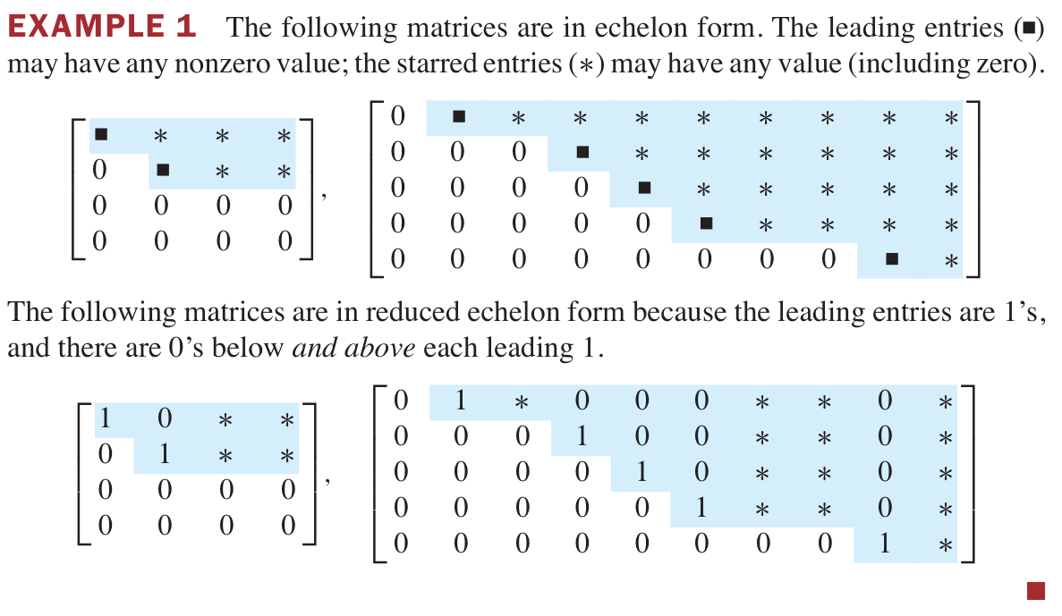
The form of is called row-echelon form, or sometimes just echelon form. To be precise: in row-echelon form, the leading entry (left-most nonzero entry) in each row is somewhere to the right of the leading entries in the rows above, and rows of only zeros are at the bottom.

The combined process of creating as in LU decomposition and then continuing pivots and eliminations to put in row-echelon form is called row reduction.

• Row-echelon form for is very useful for inversion problems (see below). – For inversion problems, we will perform row reduction simultaneously on and on a vector or matrix upon which we are inverting the action of .
• Row-echelon form for is not needed for finding determinants (see below). – Indeed, row-echelon can only differ from other triangular when the determinant is zero.

Preimages and inversion

Recall the inversion problems we are interested in, namely solving for vector or matrix in these equations:

The LU factorization, and in particular the row reduction process yielding row-echelon form, is the perfect tool to solve these equations. Replacing with , we have:

In the process of finding we actually found . Applying the action to both sides:

where and .

Now assume that is in row-echelon form. We can solve these equations for and using the second fundamental technique of this packet, called back substitution.

Just as elimination is equivalent to inverting , back substitution is equivalent to inverting . Inverting with eliminations provides the row-echelon form, and inverting with back substitutions provides the reduced row-echelon form.

Reduced row-echelon form

Given in row-echelon form, it is also in reduced row-echelon form (RREF) when the leading nonzero entries in each row are ones, and any column with a leading one has all other entries equal to zero.

Back substitution is the process of applying row-scale and row-add matrix actions to convert a matrix in REF to a matrix in RREF. This is a continuation of “row reduction,” with a difference being that the matrices performing back substitution operations are not lower triangular, they are now upper triangular. Another difference is that we don’t have good reasons (in terms of applications) to record these back substitution matrices, we simply let them act on our matrix, or simultaneously on our matrix and vector (in the case of ) or on our matrix and matrix (in the case of ).

To find the RREF of a matrix in REF, we:

Computing reduced row-echelon form from row-echelon form

• Act by row-scale matrices to change the leading entries to ones.
• Act by more row-add matrices to eliminate the entries above leading ones.

Any RREF matrix can be written in terms of block submatrices:

Here is the identity as a submatrix (the size of depends on how many zeros are in ), is some other submatrix, and are zeros filling out the rest of .

Example

Back substitution: convert REF to RREF

Exercise 09-04

Back substitution: convert REF to RREF

Convert from REF to RREF.

Preimage of a vector

The RREF of a matrix reveals the complete set of possible inverses (preimages) of a given vector.

Example

Inverting a vector using RREF

Consider the equation , with a row-reduced :

This matrix translates to the system of equations:

There is a solution vector provided . If that is true, any and can be chosen, and are quickly found by solving the system. Given any choice of and , there is only one possibility for each of . Notice that the leading ones (also called pivots) are in columns and , and and are determined. There are no pivots in columns and , and and are free to take any value.

We can go farther and write the complete set of solutions as the span of two vectors plus an offset, using values of and as the coefficients:

so we could write, if you like: .

If we wish to solve an equation and is not yet in reduced row-echelon form, then we must convert to that form, while simultaneously applying the row reductions and pivots to the vector . (This means applying the same invertible transformations to both sides of the equation.) Row reduction is easily performed on and simultaneously by combining them into the augmented matrix and row reducing this instead. (This means: create a matrix by adding as an additional column to , and put a vertical line between them to demarcate the end of .)

Example

Inverting a vector: row reduction of augmented matrix

Suppose we are trying to solve with and given by the following data:

Notice that is already in row-echelon form. So we create the augmented matrix and row-reduce it further to put into RREF:

and we discover that are free, and and . The possible solutions for are therefore:

Solving linear systems

A linear system looks something like this:

This system is easily represented as the vector inversion problem of , with and given by:

The techniques of elimination and back substitution that we have learned for matrices correspond to the techniques of the same names that you already know for solving systems of equations.

Exercise 09-05

Comparing elimination and elimination

Explain (with some details in an example) how elimination for matrices (corresponding to multiplication by for some single-column row-add combo matrix ) is equivalent to elimination for a system of equations.

Hint: solve the above system using elimination and back substitution as in high school algebra, and then solve the same system as a vector preimage problem using row reduction to RREF of the augmented matrix. Write your solution steps in corresponding order so that you can match the corresponding steps between the two methods.

Preimage of a matrix

The technique for inverting a vector can be applied to find the preimage of a matrix simply by inverting the column vectors of that matrix. Namely, given the equation:

notice that if we write and in terms of their column vectors, we have:

In principle, we can simply invert one at a time, in sequence.

In practice, a much faster way to find is to write the augmented matrix and row reduce this matrix.

The most important use of this technique is to find the inverse of an invertible matrix. Given , the inverse is found by computing the preimage of under the action of , in other words by setting and row reducing the augmented matrix .

Example

Inverse of a matrix

Problem: Find the inverse of the matrix .

Solution: We row reduce the augmented matrix using pivots, eliminations, and back substitutions to put into RREF:

Therefore we have found .

Determinants

Two facts about determinants allow us to use LU factorization to compute the determinant of any matrix:

Two determinant facts

• The determinant of any triangular matrix is equal to the product of its diagonal entries.
• The determinant is multiplicative: .

If , then , and assuming it has only ones on the diagonal. So is the product of the diagonal entries of .

If , then . It turns out that . So where again is the product of diagonal entries. The choice of sign is given by where is the number of non-trivial row-swaps that are composed to give .

Problems due 20 Mar 2024 by 9:00am

Problem 09-01

Row reduction of a product

Suppose and is invertible. Prove that any sequence of row reduction operations which reduces to will also reduce to . Can you relate this fact to the LU decomposition?

Problem 09-02

LU factorization and solving

Compute the LU factorization of :

Use this to find the unique value of that satisfies , where . (You should perform the elimination and back-substitution operations on the rows of that are dictated by the LU decomposition of .) Also: what is the determinant of ?

Problem 09-03

Inverse of using LU

Compute the inverse of from Problem 09-02 using the LU factorization computed in that problem, in other words by computing . Now compute using the method at the end of the packet: perform row reduction on the augmented matrix . Which method do you like better?

Problem 09-04

Row reduction with pivoting

Perform row reduction with pivoting upon the matrix in order to find all solutions to the equation with . (You can use the augmented matrix; no need to compute the full decomposition.)