Applied Linear Algebra - Packet 13

Packet 13

Matrices IV: Spectrum

Eigenvectors, eigenvalues: Part II

Example

Finding eigenvectors and eigenvalues

Problem: Find the eigenvectors and their eigenvalues for the matrix $A=\left(\begin{array}{ccc}4& 0& 1\\ -2& 1& 0\\ -2& 0& 1\end{array}\right)$. Solution: First find the eigenvalues:

$$\begin{array}{cc}\det A_{\lambda }& =\left|\begin{array}{ccc}4-\lambda & 0& 1\\ -2& 1-\lambda & 0\\ -2& 0& 1-\lambda \end{array}\right|\\ & \\ & =(4-\lambda )\left|\begin{array}{cc}1-\lambda & 0\\ 0& 1-\lambda \end{array}\right|-0\left|\begin{array}{cc}-2& 0\\ -2& 1-\lambda \end{array}\right|+1\left|\begin{array}{cc}-2& 1-\lambda \\ -2& 0\end{array}\right|\\ & \\ & =(4-\lambda ){(1-\lambda )}^2-0+2(1-\lambda )\\ & =-{\lambda }^3+6{\lambda }^2-11\lambda +6.\end{array}$$

The roots are $\lambda =\mathrm{1,2,3}$. (The rational roots theorem leads to the guess $\lambda =2$, and then you can divide the cubic polynomial by $\lambda -2$ to obtain a quadratic one, which is easily factored.)

Now we seek eigenvectors by solving $A_{\lambda }𝐱=\mathrm{𝟎}$ for each $\lambda$ root. When $\lambda =1$:

$$A_{\lambda }𝐱=\left(\begin{array}{ccc}3& 0& 1\\ -2& 0& 0\\ -2& 0& 0\end{array}\right)\left(\begin{array}{c}{x}_1\\ x_2\\ x_3\end{array}\right)=\left(\begin{array}{c}0\\ 0\\ 0\end{array}\right).$$

To solve for $𝐱$, row reduce $A_{\lambda }$ to obtain a matrix in RREF:

$$\begin{array}{cc}{A}_{\lambda }& =\left(\begin{array}{ccc}3& 0& 1\\ -2& 0& 0\\ -2& 0& 0\end{array}\right)\sim \left(\begin{array}{ccc}3& 0& 1\\ 0& 0& 2/3\\ 0& 0& 2/3\end{array}\right)\\ & \\ & \sim \left(\begin{array}{ccc}3& 0& 0\\ 0& 0& 2/3\\ 0& 0& 0\end{array}\right)\sim \left(\begin{array}{ccc}1& 0& 0\\ 0& 0& 1\\ 0& 0& 0\end{array}\right).\end{array}$$

So we know $x_1=x_3=0$ and $x_2$ is free. Plugging these in we have $𝐱=\left(\begin{array}{c}0\\ x_2\\ 0\end{array}\right)$, and we choose $x_2=1$ obtaining $\left(\begin{array}{c}0\\ 1\\ 0\end{array}\right)$ for an eigenvector.

Next for $\lambda =2$ we have:

$$A_{\lambda }𝐱=\left(\begin{array}{ccc}2& 0& 1\\ -2& -1& 0\\ -2& 0& -1\end{array}\right)\left(\begin{array}{c}{x}_1\\ x_2\\ x_3\end{array}\right)=\left(\begin{array}{c}0\\ 0\\ 0\end{array}\right).$$

To solve for $𝐱$, row reduce $A_{\lambda }$ to obtain a matrix in RREF:

$$\begin{array}{cc}{A}_{\lambda }& =\left(\begin{array}{ccc}2& 0& 1\\ -2& -1& 0\\ -2& 0& -1\end{array}\right)\sim \left(\begin{array}{ccc}2& 0& 1\\ 0& -1& 1\\ 0& 0& 0\end{array}\right)\sim \left(\begin{array}{ccc}1& 0& 1/2\\ 0& 1& -1\\ 0& 0& 0\end{array}\right).\end{array}$$

So we know $x_1=-\frac{1}{2}{x}_3$ and $x_2=+x_3$. Plugging these in we have $𝐱=\left(\begin{array}{c}-\frac{1}{2}{x}_3\\ x_3\\ x_3\end{array}\right)$, and we choose $x_3=2$ obtaining $\left(\begin{array}{c}-1\\ 2\\ 2\end{array}\right)$.

Finally for $\lambda =3$ we have:

$$A_{\lambda }𝐱=\left(\begin{array}{ccc}1& 0& 1\\ -2& -2& 0\\ -2& 0& -2\end{array}\right)\left(\begin{array}{c}{x}_1\\ x_2\\ x_3\end{array}\right)=\left(\begin{array}{c}0\\ 0\\ 0\end{array}\right).$$

To solve for $𝐱$, row reduce $A_{\lambda }$ to obtain a matrix in RREF:

$$\begin{array}{cc}{A}_{\lambda }& =\left(\begin{array}{ccc}1& 0& 1\\ -2& -2& 0\\ -2& 0& -2\end{array}\right)\sim \left(\begin{array}{ccc}1& 0& 1\\ 0& -2& 2\\ 0& 0& 0\end{array}\right)\sim \left(\begin{array}{ccc}1& 0& 1\\ 0& 1& -1\\ 0& 0& 0\end{array}\right).\end{array}$$

So we know $x_1=-x_3$ and $x_2=+x_3$. Plugging these in we have $𝐱=\left(\begin{array}{c}-x_3\\ x_3\\ x_3\end{array}\right)$, and we choose $x_3=1$ obtaining $\left(\begin{array}{c}-1\\ 1\\ 1\end{array}\right)$.

Example

Changing to eigenbasis yields diagonal matrix

Notice that $A$ in the previous example has three eigenvectors, and that they are independent. Therefore they constitute a basis of ${ℝ}^3$; let’s call this basis $𝒞$. Putting these basis vectors as the columns of a matrix, we create the change of basis transfer matrix from $𝒞$ to the standard basis $ℬ$:

$${}_{ℬ}{T}_{𝒞}=\left(\begin{array}{ccc}{𝐜}_1& {𝐜}_2& {𝐜}_3\end{array}\right)=\left(\begin{array}{ccc}0& -1& -1\\ 1& 2& 1\\ 0& 2& 1\end{array}\right).$$

So ${}_{ℬ}{T}_{𝒞}\cdot {[𝐱]}_{𝒞}=x_1{𝐜}_1+x_2{𝐜}_2+x_3{𝐜}_3=x_1\left(\begin{array}{c}0\\ 1\\ 0\end{array}\right)+x_2\left(\begin{array}{c}-1\\ 2\\ 2\end{array}\right)+x_3\left(\begin{array}{c}-1\\ 1\\ 1\end{array}\right)$.

Now consider that these are eigenvectors of $A$ with eigenvalues $\mathrm{1,2,3}$:

$$A{𝐜}_1={𝐜}_1,A{𝐜}_2=2{𝐜}_2,A{𝐜}_3=3{𝐜}_3.$$

If we write $A$ in the basis $𝒞$ using the transfer matrix ${}_{ℬ}{T}_{𝒞}$, we have:

$$\begin{array}{cc}{[A]}_{𝒞}& ={\phantom{}}_{𝒞}{T}_{ℬ}\cdot A\cdot {\phantom{}}_{ℬ}{T}_{𝒞}\\ & \\ & ={\left(\begin{array}{ccc}0& -1& -1\\ 1& 2& 1\\ 0& 2& 1\end{array}\right)}^{-1}\left(\begin{array}{ccc}4& 0& 1\\ -2& 1& 0\\ -2& 0& 1\end{array}\right)\left(\begin{array}{ccc}0& -1& -1\\ 1& 2& 1\\ 0& 2& 1\end{array}\right)=\left(\begin{array}{ccc}1& 0& 0\\ 0& 2& 0\\ 0& 0& 3\end{array}\right).\end{array}$$

In other words, the matrix of $A$ is a diagonal matrix when written in the basis of its own eigenvectors.

The example above illustrates a general fact: if a matrix $A$ has enough independent eigenvectors $\{{𝐜}_1,\dots ,{𝐜}_n\}$ to form a basis of the vector space ${ℝ}^n$ on which $A$ acts, then if you write $A$ in the basis of these eigenvectors, it will have a diagonal form.

In other words, the eigenbasis of $A$ is a natural basis for $A$. It is a basis in which the action of $A$ is extremely simple: it is given by scaling the basis vectors by the respective eigenvalue numbers.

Sometimes a matrix has not enough independent eigenvectors. Here is an illustration:

Example

Matrix with too few eigenvectors

The matrix $A=\left(\begin{array}{cc}1& 1\\ 0& 1\end{array}\right)$ has $\det A_{\lambda }={(1-\lambda )}^2$. Therefore it has a “double” eigenvalue $\lambda =+1$. To find the eigenvectors:

$$A_{+1}\cdot 𝐱=\left(\begin{array}{cc}0& 1\\ 0& 0\end{array}\right)\left(\begin{array}{c}{x}_1\\ x_2\end{array}\right)=\left(\begin{array}{c}0\\ 0\end{array}\right).$$

The matrix is already in RREF. So the equation says that $x_1$ is free and $x_2=0$. Therefore we have the eigenvector $\left(\begin{array}{c}1\\ 0\end{array}\right)$.

However, no more eigenvectors are available (other than scalar multiples of this one, which would not be independent of this one). Therefore it is impossible to find a basis of eigenvectors, and it is thus impossible to convert $A$ to diagonal form by a change of basis.

Sometimes a real matrix has complex eigenvalues and eigenvectors. Here is an illustration:

Example

Matrix with complex eigenvalues and eigenvectors

The matrix $A=\left(\begin{array}{cc}0& -1\\ 1& 0\end{array}\right)$ has $\det A_{\lambda }={\lambda }^2+1$ so its eigenvalues are $\lambda =\pm i$. To find the eigenvectors:

$$A_i\cdot 𝐱=\left(\begin{array}{cc}-i& -1\\ 1& -i\end{array}\right)\left(\begin{array}{c}{x}_1\\ x_2\end{array}\right)=\left(\begin{array}{c}0\\ 0\end{array}\right).$$

Row reduce the matrix $A_i$:

$$A_i=\left(\begin{array}{cc}-i& -1\\ 1& -i\end{array}\right)\sim \left(\begin{array}{cc}-i& -1\\ 0& 0\end{array}\right)\sim \left(\begin{array}{cc}1& -i\\ 0& 0\end{array}\right).$$

This is now in RREF, so we see that $x_1=i{x}_2$ and $x_2$ is free, so we get the eigenvector $\left(\begin{array}{c}i\\ 1\end{array}\right)$.

Following the same procedure for $\lambda =-i$, we find the eigenvector $\left(\begin{array}{c}-i\\ 1\end{array}\right)$.

It is important to be aware of these two situations. For the sake of exams, you should memorize one example of each type. (You can use the two above.)

Question 13-01

Double eigenvalues does not imply insufficient eigenvectors

What are the eigenvalues and eigenvectors of $A=\left(\begin{array}{cc}2& 0\\ 0& 2\end{array}\right)$? Are there enough to form a basis of ${ℝ}^2$?

Question 13-02

Enough eigenvectors?

Does the matrix $A=\left(\begin{array}{ccc}2& 1& 0\\ 0& 2& 1\\ 0& 0& 2\end{array}\right)$ have enough eigenvectors to form a basis? If not, how many does it have?

Spectral Theorem: symmetric matrices have good eigen theory

A key point of the Spectral Theorem is that symmetric matrices never encounter the phenomena illustrated in the two examples above. Eigenvalues are always real numbers, and there are always enough eigenvectors to form a basis.

Eigenvectors vs. singular vectors

It is helpful to think about the concept of an eigenvector as consisting of two aspects:

• (1) Matrix acting by scaling
• (2) Fixed lines of matrix action

Aspect (1) allows easy computation and geometric understanding of the matrix action. It also allows us to focus on vectors that are more important (those having a larger scale factor). If we have a basis of such vectors, the matrix will have a simple diagonal form when written in this basis.

Aspect (2) goes much further, even though it essentially includes aspect (1). A fixed line (eigenline) is the span of any eigenvector. Such lines are mapped to themselves by the matrix action. This aspect describes eigenvector spans as analogues of fixed points of a function. The concept of fixed points and fixed lines (‘fixity’ in general) only applies when the function or matrix keeps vectors in the same space, i.e. has the same codomain as domain.

Eigenvectors There are various contexts where a matrix does act on vectors in a single space. Aspect (2) is very useful in these contexts. For example, a differential operator, which produces a system of first-order linear differential equations, involves a matrix $A:V\to V$ for a vector space of functions $V$. For another example, the moment of inertia matrix describing angular moment of $3$D bodies in physics. Or the many operators of quantum mechanics.

One of the biggest advantages of aspect (2) is that it is compatible with iteration.

If $A:V\to V$ is a linear transformation (i.e. a matrix) having the same codomain as domain, we can define iterates $A^2,A^3$ etc. as matrix powers. These powers allow one to apply functions to matrices: if $f(x)={\sum }_{n=0}^{\infty }{a}_n{x}^n$ is a power series, we can define $f(A)$ by the power series $f(A)={\sum }_{n=0}^{\infty }{a}_n{A}^n$. (Bracketing any problems with convergence.) An extremely important series is $e^x=1+x+\frac{x^2}{2!}+\frac{x^3}{3!}+\cdots$, since the function $e^{At}$ solves the linear ODE system $X^{\prime }(t)=AX(t)$.

It is hard to compute $e^{At}$, or more generally ${\sum }_{n=0}^{\infty }{a}_n{A}^n$, by direct multiplication and limits of partial sums. On the other hand, it is easy to compute $e^{At}$ when $A$ is a diagonal matrix, just as it is easy to compute $A^2𝐯$ when $𝐯$ is an eigenvector of $A$. (Namely, the latter is ${\lambda }^2𝐯$.) For example, in the $2\times 2$ case we have $e^{\left(\begin{array}{cc}{\lambda }_1& 0\\ 0& {\lambda }_2\end{array}\right)}=\left(\begin{array}{cc}{e}^{{\lambda }_1}& 0\\ 0& e^{{\lambda }_2}\end{array}\right)$.

Even when $A$ is not diagonal, if an eigenbasis matrix ${\phantom{}}_{ℬ}{T}_{𝒞}=\left(\begin{array}{cccc}{𝐜}_1& {𝐜}_2& \dots & {𝐜}_n\end{array}\right)$ can be found, then the powers of $A$ are still easy to calculate, because (e.g. in $3$D):

$$\begin{array}{cc}{A}^2& ={\phantom{}}_{ℬ}{T}_{𝒞}\left(\begin{array}{ccc}{\lambda }_1& 0& 0\\ 0& {\lambda }_2& 0\\ 0& 0& {\lambda }_3\end{array}\right){\phantom{}}_{𝒞}{T}_{ℬ}{\phantom{}}_{ℬ}{T}_{𝒞}\left(\begin{array}{ccc}{\lambda }_1& 0& 0\\ 0& {\lambda }_2& 0\\ 0& 0& {\lambda }_3\end{array}\right){\phantom{}}_{𝒞}{T}_{ℬ}\\ & \\ & ={\phantom{}}_{ℬ}{T}_{𝒞}\left(\begin{array}{ccc}{\lambda }_1& 0& 0\\ 0& {\lambda }_2& 0\\ 0& 0& {\lambda }_3\end{array}\right){\phantom{}}_{ℬ}{T}_{𝒞}^{-1}{\phantom{}}_{ℬ}{T}_{𝒞}\left(\begin{array}{ccc}{\lambda }_1& 0& 0\\ 0& {\lambda }_2& 0\\ 0& 0& {\lambda }_3\end{array}\right){\phantom{}}_{𝒞}{T}_{ℬ}\\ & \\ & ={\phantom{}}_{ℬ}{T}_{𝒞}\left(\begin{array}{ccc}{\lambda }_1& 0& 0\\ 0& {\lambda }_2& 0\\ 0& 0& {\lambda }_3\end{array}\right)\left(\begin{array}{ccc}{\lambda }_1& 0& 0\\ 0& {\lambda }_2& 0\\ 0& 0& {\lambda }_3\end{array}\right){\phantom{}}_{𝒞}{T}_{ℬ}\\ & \\ & ={\phantom{}}_{ℬ}{T}_{𝒞}\left(\begin{array}{ccc}{\lambda }_1^2& 0& 0\\ 0& {\lambda }_2^2& 0\\ 0& 0& {\lambda }_3^2\end{array}\right){\phantom{}}_{𝒞}{T}_{ℬ}.\end{array}$$

Similarly we have:

$$A^n={\phantom{}}_{ℬ}{T}_{𝒞}\left(\begin{array}{ccc}{\lambda }_1^n& 0& 0\\ 0& {\lambda }_2^n& 0\\ 0& 0& {\lambda }_3^n\end{array}\right){\phantom{}}_{𝒞}{T}_{ℬ},e^A={\phantom{}}_{ℬ}{T}_{𝒞}\left(\begin{array}{ccc}{e}^{{\lambda }_1}& 0& 0\\ 0& e^{{\lambda }_2}& 0\\ 0& 0& e^{{\lambda }_3}\end{array}\right){\phantom{}}_{𝒞}{T}_{ℬ}.$$

The critical piece of the calculation above is the cancellation ${\phantom{}}_{ℬ}{T}_{𝒞}^{-1}{\phantom{}}_{ℬ}{T}_{𝒞}=I_3$ occurring in the calculation for $A^2$. This cancellation shows that matrix multiplication and change of basis can be performed in either order. That in turn means we can first change basis to an eigenbasis (if it exists) and then perform multiplication with the diagonal matrices where it is easy, and only afterwards change back to the standard basis.

Singular vectors The concept of singular vector is designed to make use of aspect (1) of eigenvectors without aspect (2). Because they do not include aspect (2), singular vectors of $A$ are not eigenvectors of $A$ except in special cases. They do not determine fixed lines of the $A$ action.

Unlike eigenvectors and eigenvalues, singular vectors and singular values are (best) defined in the context of a collection of vectors giving the singular value decomposition (SVD). So, a singular vector is one of the vectors in the SVD.

Defining the singular value decomposition

Suppose $A:{ℝ}^n\to {ℝ}^m$ is a matrix providing a linear transformation between different vector spaces.

SVD features

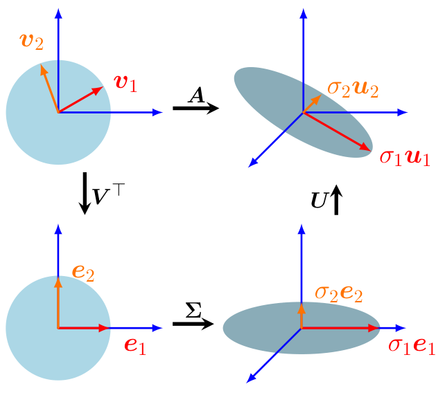
A singular value decomposition of $A:{ℝ}^n\to {ℝ}^m$ is given by: $A=U\mathrm{\Sigma }{V}^{𝖳},$ where:

• $V=\left(\begin{array}{cccc}{𝐯}_1& {𝐯}_2& \cdots & {𝐯}_n\end{array}\right)$ is an orthogonal matrix giving a rotation/reflection combo for ${ℝ}^n$ (input)
• $U=\left(\begin{array}{cccc}{𝐮}_1& {𝐮}_2& \cdots & {𝐮}_m\end{array}\right)$ is an orthogonal matrix giving a rotation/reflection combo for ${ℝ}^m$ (output)
• $\mathrm{\Sigma }$ has non-negative entries ${\sigma }_1,{\sigma }_2,\dots {\sigma }_{\ell }$ on the main diagonal (possibly zeros!) and zeros elsewhere. (Here $\ell =\min \{n,m\}$.) It is not square if $n\ne m$. It could look like these, for example:

$$\left(\begin{array}{cccc}1& 0& 0& 0\\ 0& 3& 0& 0\\ 0& 0& 7& 0\\ 0& 0& 0& 0\\ 0& 0& 0& 0\end{array}\right),\left(\begin{array}{cccccc}1& 0& 0& 0& 0& 0\\ 0& 3& 0& 0& 0& 0\\ 0& 0& 7& 0& 0& 0\end{array}\right).$$

The orthonormal basis vectors ${𝐯}_1,\dots ,{𝐯}_n$ are called right singular vectors. The orthonormal basis vectors ${𝐮}_1,\dots ,{𝐮}_m$ are called left singular vectors. The values ${\sigma }_i\ge 0$ are the lengths of the images, namely ${\sigma }_i=|A{𝐯}_i|$.

(Remember: “Right $=$ Input, Left $=$ Output.”)

An alternate way to write the SVD uses scalar projections ${𝐯}_i^{𝖳}$ attached to the vectors ${𝐮}_i$:

$$A={\sigma }_1{𝐮}_1{𝐯}_1^{𝖳}+{\sigma }_2{𝐮}_2{𝐯}_2^{𝖳}+\cdots +{\sigma }_{\ell }{𝐮}_{\ell }{𝐯}_{\ell }^{𝖳}.$$

Each term ${\sigma }_i{𝐮}_i{𝐯}_i^{𝖳}$ takes an input vector, dots it with ${𝐯}_i$, then applies this value to ${𝐮}_i$ scaled by ${\sigma }_i$. With this formula, we can compute $A𝐱$ for any input $𝐱$ using dot products:

$$A𝐱={\sigma }_1{𝐮}_1({𝐯}_1\cdot 𝐱)+{\sigma }_2{𝐮}_2({𝐯}_2\cdot 𝐱)+\cdots +{\sigma }_{\ell }{𝐮}_{\ell }({𝐯}_{\ell }\cdot 𝐱).$$

By plugging in $𝐱={𝐯}_i$, we verify that $A{𝐯}_1={\sigma }_1{𝐮}_1$ and $A{𝐯}_2={\sigma }_2{𝐮}_2$, etc. up to $A{𝐯}_{\ell }={\sigma }_{\ell }{𝐮}_{\ell }$. (For $\ell <i\le n$, we have $A{𝐯}_i=\mathrm{𝟎}$.)

Singular vectors vs. eigenvectors

The rule $A{𝐯}_i={\sigma }_i{𝐮}_i$ looks analogous to the rule for eigenvectors.

But it’s actually very different! Notice that ${𝐯}_i$ and ${𝐮}_i$ are not even vectors in the same space!

The rule $A𝐯=\sigma 𝐮$ does not by itself determine any special property of $𝐯$ or $𝐮$. (Take any unit vector $𝐯$, apply $A$, then define $𝛔=|A𝐯|$ and $𝐮={\sigma }^{-1}A𝐯$.)

The significance of the rule $A{𝐯}_i={\sigma }_i{𝐮}_i$ manifests when it holds simultaneously on all vector pairs in orthonormal bases ${𝐯}_1,\dots ,{𝐯}_n$ and ${𝐮}_1,\dots ,{𝐮}_m$.

Still, the SVD says that after rotating / reflecting the basis of ${ℝ}^n$ and the basis of ${ℝ}^m$ by suitable orthogonal matrices (not necessarily the same on each), the action of $A$ can be represented as simple scalings by ${\sigma }_i$.

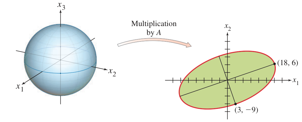
We may think of ${𝐯}_1,\dots ,{𝐯}_n$ as a special basis for the input space ${ℝ}^n$ vis-à-vis the matrix $A$, and ${𝐮}_1,\dots ,{𝐮}_m$ as a corresponding basis for the output space ${ℝ}^m$. Then $A$ acts by pairing the vector ${𝐯}_i$ to ${𝐮}_i$ and stretching it by ${\sigma }_i$.

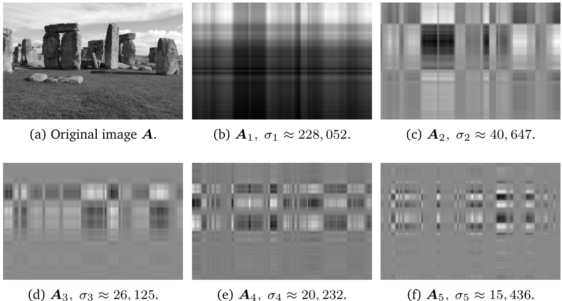Partial matrices ${𝐮}_i{𝐯}_i^{𝖳}$ for $i=1,\dots ,5$.

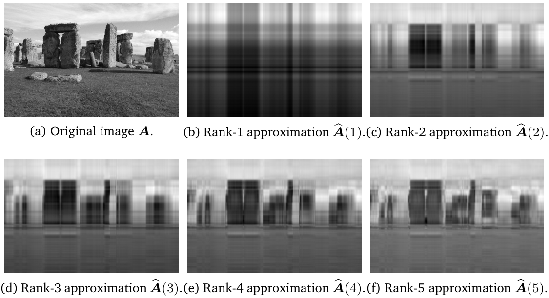Partial sum matrices ${\sigma }_1{𝐮}_1{𝐯}_1^{𝖳}+\cdots +{\sigma }_i{𝐮}_i{𝐯}_i^{𝖳}$ for $i=1,\dots ,5$.

Computing the singular value decomposition

In practice, on a computer, the SVD is calculated using numerical procedures that are akin to those used to find approximations to eigenvectors. We do not address those kinds of procedures in this course.

Still, it is possible to specify and calculate SVD elements by hand for a matrix $A$ by making use of the fact that $A^{𝖳}A$ is always a symmetric matrix and the Spectral Theorem can be applied to it. This method also shows that the SVD always exists, since the symmetric $A^{𝖳}A$ always has real eigenvalues and enough eigenvectors by the Spectral Theorem, even when $A$ does not. Let us see how this works.

First observe that $(A^{𝖳}A{)}^{𝖳}=A^{𝖳}(A^{𝖳}{)}^{𝖳}=A^{𝖳}A$, so $A^{𝖳}A$ is always symmetric. Also notice that $A^{𝖳}A:{ℝ}^n\to {ℝ}^n$, so the input and output spaces of this matrix are the same.

SVD elements

• ${𝐯}_1,\dots ,{𝐯}_n=$ orthonormal eigenbasis of $A^{𝖳}A$. $$ As guaranteed by the Spectral Theorem, so $V$ here is $Q$ in the notation of that theorem.
• ${\sigma }_i=|A{𝐯}_i|$ defined for $1\le i\le \ell$. $$ If $\left(A^{𝖳}A\right){𝐯}_i={\lambda }_i{𝐯}_i$, then ${\sigma }_i=\sqrt{{\lambda }_i}$.
• The equation ${\sigma }_i{𝐮}_i=A{𝐯}_i$ for $1\le i\le \ell$ defines unit vectors ${𝐮}_i$ for those $i$ with ${\sigma }_i\ne 0$.
• Gram-Schmidt provides additional ${𝐮}_i$ vectors when ${\sigma }_i=0$.

Example

Computing SVD by hand

Problem: Find an SVD for the matrix $A=\left(\begin{array}{cc}1& -1\\ -2& 2\\ 2& -2\end{array}\right)$.

Solution: First calculate that $A^{𝖳}A=\left(\begin{array}{cc}9& -9\\ -9& 9\end{array}\right)$ and this matrix has $\lambda =18$ and $\lambda =0$ eigenvalues. Therefore we set ${\sigma }_1=3\sqrt{2}$ and ${\sigma }_2=0$. By solving $\left(\begin{array}{cc}-9& -9\\ -9& -9\end{array}\right)\left(\begin{array}{c}{x}_1\\ x_2\end{array}\right)=\left(\begin{array}{c}0\\ 0\end{array}\right)$ we obtain an eigenvector $\left(\begin{array}{c}1\\ -1\end{array}\right)$ which we renormalize to the unit vector $\left(\begin{array}{c}1/\sqrt{2}\\ -1/\sqrt{2}\end{array}\right)$. By solving $\left(\begin{array}{cc}9& -9\\ -9& 9\end{array}\right)\left(\begin{array}{c}{x}_1\\ x_2\end{array}\right)=\left(\begin{array}{c}0\\ 0\end{array}\right)$ we obtain an eigenvector $\left(\begin{array}{c}1\\ 1\end{array}\right)$ which we renormalize to the unit vector $\left(\begin{array}{c}1/\sqrt{2}\\ 1/\sqrt{2}\end{array}\right)$. We now have $V$ and $\mathrm{\Sigma }$:

$$\mathrm{\Sigma }=\left(\begin{array}{cc}3\sqrt{2}& 0\\ 0& 0\\ 0& 0\end{array}\right),V=\left(\begin{array}{cc}1/\sqrt{2}& 1/\sqrt{2}\\ -1/\sqrt{2}& 1/\sqrt{2}\end{array}\right).$$

Set

$${𝐮}_1={\sigma }_1^{-1}A{𝐯}_1=\frac{1}{3\sqrt{2}}\left(\begin{array}{c}2/\sqrt{2}\\ -4/\sqrt{2}\\ 4/\sqrt{2}\end{array}\right)=\left(\begin{array}{c}1/3\\ -2/3\\ 2/3\end{array}\right)$$

and we notice that $|{𝐮}_1|=1$. Now we need ${𝐮}_2,{𝐮}_3$ unit vectors orthogonal to each other and to ${𝐮}_1$. We first calculate a span of the kernel of the matrix ${𝐮}_1^{𝖳}$, and then perform Gram-Schmidt to orthogonalize it. For the kernel:

$$\left(\begin{array}{ccc}1/3& -2/3& 2/3\end{array}\right)\left(\begin{array}{c}{x}_1\\ x_2\\ x_3\end{array}\right)=0,$$

and therefore $x_1-2x_2+2x_3=0$ so we can set $x_2,x_3$ free and solve for $x_1$, thereby obtaining generators for the kernel:

$$\ker {𝐮}_1^{𝖳}=\{\left(\begin{array}{c}2x_2-2x_3\\ x_2\\ x_3\end{array}\right)\}=⟨{𝐰}_2=\left(\begin{array}{c}2\\ 1\\ 0\end{array}\right),{𝐰}_3=\left(\begin{array}{c}-2\\ 0\\ 1\end{array}\right)⟩.$$

Now we already have ${𝐰}_2⟂{𝐮}_1$ by our method of defining ${𝐰}_2$. So it just remains to do the last step of Gram-Schmidt. We calculate that

$${𝐰}_3-\frac{{𝐰}_3\cdot {𝐮}_1}{{𝐮}_1\cdot {𝐮}_1}{𝐮}_1-\frac{{𝐰}_3\cdot {𝐰}_2}{{𝐰}_2\cdot {𝐰}_2}{𝐰}_2=\left(\begin{array}{c}-2\\ 0\\ 1\end{array}\right)-\frac{0}{1}\left(\begin{array}{c}1/3\\ -2/3\\ 2/3\end{array}\right)-\frac{-4}{5}\left(\begin{array}{c}2\\ 1\\ 0\end{array}\right)=\left(\begin{array}{c}-2/5\\ 4/5\\ 1\end{array}\right).$$

Then

$${𝐮}_2=\frac{1}{|{𝐰}_2|}{𝐰}_2=\left(\begin{array}{c}2/\sqrt{5}\\ 1/\sqrt{5}\\ 0\end{array}\right),{𝐮}_3=\frac{5}{\sqrt{45}}\left(\begin{array}{c}-2/5\\ 4/5\\ 1\end{array}\right)=\left(\begin{array}{c}-2/\sqrt{45}\\ 4/\sqrt{45}\\ 5/\sqrt{45}\end{array}\right).$$

We have finished, and the SVD is given by:

$$A=U\mathrm{\Sigma }{V}^{𝖳}=\left(\begin{array}{ccc}1/3& 2/\sqrt{5}& -2/\sqrt{45}\\ -2/3& 1/\sqrt{5}& 4/\sqrt{45}\\ 2/3& 0& 5/\sqrt{45}\end{array}\right)\left(\begin{array}{cc}3\sqrt{2}& 0\\ 0& 0\\ 0& 0\end{array}\right)\left(\begin{array}{cc}1/\sqrt{2}& -1/\sqrt{2}\\ 1/\sqrt{2}& 1/\sqrt{2}\end{array}\right).$$

Exercise 13-01

Computing SVD by hand

Find an SVD for the matrix $A=\left(\begin{array}{cc}2& -1\\ 2& 2\end{array}\right)$.

Exercise 13-02

Computing SVD by hand

Find an SVD for the matrix $A=\left(\begin{array}{cc}-3& 1\\ 6& -2\\ 6& -2\end{array}\right)$.

Explaining the SVD elements

First, why is $V=\left(\begin{array}{ccc}{𝐯}_1& \dots & {𝐯}_n\end{array}\right)$ an orthogonal matrix? $$ Answer: Since ${𝐯}_1,\dots ,{𝐯}_n$ is an orthonormal basis, the matrix $V$ is orthogonal. Second, why is $U=\left(\begin{array}{ccc}{𝐮}_1& \dots & {𝐮}_m\end{array}\right)$ an orthogonal matrix? $$ Answer: Consider the calculation:

$$\begin{array}{cc}⟨A{𝐯}_i,A{𝐯}_j⟩& ={(A{𝐯}_i)}^{𝖳}A{𝐯}_j\\ & ={𝐯}_i^{𝖳}{A}^{𝖳}A{𝐯}_j\\ & ={𝐯}_i^{𝖳}(A^{𝖳}A{𝐯}_j)\\ & ={𝐯}_i^{𝖳}({\lambda }_j{𝐯}_j)\\ & ={\lambda }_j({𝐯}_i^{𝖳}{𝐯}_j)\\ & =\{\begin{array}{cc}{\lambda }_j& i=j\\ 0& i\ne j.\end{array}\end{array}$$

$$ Notes: The first line is the dot product using ‘inner product’ notation. The second line is the transpose rule. The fourth line is the definition of ${𝐯}_j$ as eigenvector of $A^{𝖳}A$. The last line is the property that ${𝐯}_1,\dots ,{𝐯}_n$ are orthonormal vectors.

$$ From this calculation it follows that $A{𝐯}_1,\dots ,A{𝐯}_n$ are orthogonal vectors (at least when they aren’t zero). Since ${𝐮}_1,\dots ,{𝐮}_m$ are the same vectors renormalized as unit vectors, we know ${𝐮}_1,\dots {𝐮}_m$ are orthonormal (at least when ${\sigma }_i\ne 0$). In the case of ${\sigma }_i=|A{𝐯}_i|=0$, the alternate definition of ${𝐮}_i$ using Gram-Schmidt implies that all ${𝐮}_1,\dots ,{𝐮}_m$ are orthonormal.

Third, why is ${\sigma }_i=\sqrt{{\lambda }_i}$? $$ Answer: According to the calculation above, $|A{𝐯}_i{|}^2={\lambda }_i$. But $|A{𝐯}_i|={\sigma }_i$ by definition.

Fourth, why is $A=U\mathrm{\Sigma }{V}^{𝖳}$, with these definitions of $U,\mathrm{\Sigma },V$? $$ Answer: To verify the equality $A=U\mathrm{\Sigma }{V}^{𝖳}$, it is sufficient to verify that the matrices on both sides have the same action on a basis of ${ℝ}^n$. (If that is true, then by linearity the matrices have the same action on any vector, and therefore they are the same matrices.)

$$ Therefore, it is sufficient to verify the equality of actions on the basis ${𝐯}_1,\dots {𝐯}_n$. Since this basis is orthonormal, we see that $V^{𝖳}{𝐯}_i$ is the vector with $1$ in the $i^{\text{th}}$ row and zeros elsewhere. Then $\mathrm{\Sigma }\left(V^{𝖳}{𝐯}_i\right)$ is the $i^{\text{th}}$ column of $\mathrm{\Sigma }$, which has ${\sigma }_i$ in the $i^{\text{th}}$ row and zeros elsewhere. Finally $U\left(\mathrm{\Sigma }{V}^{𝖳}{𝐯}_i\right)$ is the $i^{\text{th}}$ row of $U$ (which is ${𝐮}_i$) scaled by ${\sigma }_i$. Therefore $\left(U\mathrm{\Sigma }{V}^{𝖳}\right){𝐯}_i={\sigma }_i{𝐮}_i$, and this is equal to $A{𝐯}_i$. All these statements are valid for $i=1,\dots ,\ell$. For $\ell <i$, both sides send ${𝐯}_i$ to $\mathrm{𝟎}$.

Backwards: Going from SVD to eigenvectors-eigenvalues of $A^{𝖳}A$

Addendum. If we already have an SVD given by $A=U\mathrm{\Sigma }{V}^{𝖳}$, with ${\sigma }_1,\dots ,{\sigma }_{\ell }$ on the diagonal of $\mathrm{\Sigma }$, then ${𝐯}_1,\dots {𝐯}_n$ must be the eigenvectors of $A^{𝖳}A$, and ${\sigma }_1^2,\dots ,{\sigma }_{\ell }^2,0,\dots ,0$ are the corresponding eigenvalues.

Proof: Observe that

$$\begin{array}{cc}{A}^{𝖳}A& ={(V^{𝖳})}^{𝖳}{\mathrm{\Sigma }}^{𝖳}{U}^{𝖳}U\mathrm{\Sigma }{V}^{𝖳}\\ & =V{\mathrm{\Sigma }}^{𝖳}{I}_n\mathrm{\Sigma }{V}^{𝖳}\\ & =V{\mathrm{\Sigma }}^{𝖳}\mathrm{\Sigma }{V}^{𝖳}\\ & =V{\mathrm{\Sigma }}^{\prime }{V}^{𝖳},\end{array}$$

where ${\mathrm{\Sigma }}^{\prime }$ is the square diagonal matrix with diagonal entries given by ${\sigma }_1^2,\dots ,{\sigma }_{\ell }^2$. Applying the matrix $A{\mathrm{\Sigma }}^{\prime }{V}^{𝖳}$ to ${𝐯}_1,\dots ,{𝐯}_{\ell }$ returns ${\sigma }_1^2{𝐯}_1,\dots ,{\sigma }_{\ell }{𝐯}_{\ell }$, which verifies the claim. (Again both matrices send ${𝐯}_i$ to $0$ for $\ell <i\le n$.)

Problems due 18 Apr 2024 by 12:00pm

Problem 13-01

Computing SVD

Compute an SVD of the matrix $A=\left(\begin{array}{cc}7& 1\\ 5& 5\\ 0& 0\end{array}\right)$.

Problem 13-02

SVD of $A^{𝖳}$

• (a) Given an SVD $A=U\mathrm{\Sigma }{V}^{𝖳}$, what is a formula for an SVD of $A^{𝖳}$? What are the singular values of $A^{𝖳}$?
• (b) Compute an SVD of the matrix $A=\left(\begin{array}{ccc}3& 2& 2\\ 2& 3& -2\end{array}\right)$ by first computing an SVD of $A^{𝖳}$ and then applying your result in (a).

Problem 13-03

Optimizing $|A𝐱|$ using singular values

• (a) Verify that $|A𝐱{|}^2=Q(𝐱)$ where $Q(𝐱)$ is the quadratic form of $A^{𝖳}A$.
• (b) Suppose $A=\left(\begin{array}{cc}4& 6\\ 0& 4\end{array}\right)$. Starting with the observation in (a), find a unit vector $𝐱$ that maximizes the value of $|A𝐱|$ (and hence of $|A𝐱{|}^2)$. Describe your answer in terms of singular values and singular vectors of $A$.

Problem 13-04

Optimizing $|A𝐱|$ to find singular vectors

Show that the second largest singular value of $A$ is equal to the maximum of $|A𝐱|$ where $𝐱$ varies over all unit vectors which are orthogonal to $𝐯$, where $𝐯$ is a right singular vector corresponding to the largest singular value of $A$.

(Notation clarification: if the singular values are listed in order of size ${\sigma }_1\ge {\sigma }_2\ge {\sigma }_3\ge \cdots \ge {\sigma }_{\ell }$, then the largest singular value is ${\sigma }_1$, the second largest is ${\sigma }_2$, and the right singular vector in the problem is ${𝐯}_1$ satisfying $A{𝐯}_1={\sigma }_1{𝐮}_1$.)

Problem 13-05

Computing SVD

Compute an SVD of the matrix $A=\left(\begin{array}{cccc}-18& 13& -4& 4\\ 2& 19& -4& 12\\ -14& 11& -12& 8\\ -2& 21& 4& 8\end{array}\right)$. You may use a calculator or computer, but you must show the steps of computation as in the Examples in this packet.