Applied Linear Algebra - Packet 14

Packet 14

Application I: Least squares and linear regression

Least squares

Recall that one application of Gram-Schmidt is to compute the distance from a vector to a subspace that is given as the span . First we compute an orthogonal basis . Then define the projection:

Finally, define , and the distance is given by .

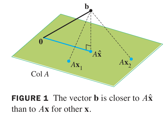
The closest point in to the vector is the projection . So the distance from to means the distance from to the closest point in , and this is the same as the magnitude of the displacement (difference) vector .

The least squares problem (or ‘LLS’ for ‘Linear Least Squares’) is the problem of finding the value of that minimizes the quantity , where is a given vector, and a given matrix.

Sometimes the least-squares solution is called the best solution to an inconsistent system. It may happen that has no solutions , for example when has small rank relative to the dimension of the vector . When there are no solutions , the system of equations that represents is called an inconsistent system. The least-squares solution is the best approximate solution, in the sense that is made as close as possible to .

‘Least squares’

The terminology ‘least squares’ is used because the minimum of occurs for the same as the minimum of , and the latter can be written as a sum of squares. For example, if and , then:

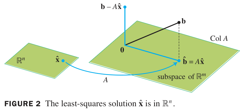
When varying over all possible input vectors, the output varies over the image (aka ‘column space’) of . Therefore, the least squares problem is the same as the problem of finding the projection of to the column space of , and then finding an which is sent by to this projection.

The column space of is the span of columns of . Therefore, one valid method is to perform Gram-Schmidt to compute the projection , and then to solve the matrix equation .

Another valid method, usually faster, makes use of some calculations in matrix algebra:

Vectors that minimize are the same as vectors that solve

First we consider an (equivalent) rearrangement of the proposed equation:

Recall that occurs if and only if is perpendicular to the columns (and hence to the image) of .

So the proposed equation holds for if and only if is perpendicular to the image of .

On the other hand, the projection is the unique vector within such that is perpendicular to . Therefore:

The least-squares error is the minimum value of . To find this error, first find the minimizing and then compute this quantity directly.

Compare: Projection Method vs.

We have two methods of finding vectors that minimize .

First method: Perform Gram-Schmidt on and then compute the projection of to the span using the orthogonal basis you found with Gram-Schmidt. This vector can be used immediately to find the least-squares error, or plugged into the second equation to solve for .

Second method: Compute the matrix and vector first, and then solve the matrix equation for possible . All solutions minimize the least-squares error, and can be plugged into to find that error.

Question: Which method is better?

Answer: If has orthogonal columns, then the projections method is better. Otherwise the equation is better.

Reason: When has orthogonal columns, Gram-Schmidt can be skipped, and the projection calculated directly. Furthermore, the scalar projections are the components on columns of – and these are exactly the components of . The projection method is much less efficient except in this simple case of orthogonal columns.

Example

Computing least-squares solution: non-orthogonal case

Problem: Consider the matrix equation There is no exact solution; find the best approximate “least-squares” solution and the resulting error.

Solution: Write and for the matrix and vector. Next calculate , and . Now solve the matrix equation We use row-reduction on the augmented matrix:

Therefore and .

To compute the error, first find :

and then subtract from and compute the norm:

Many solutions possible

If the null space of is not just the zero vector, then elements of the null space may be added to any best approximate solution without changing the output . So the linear least-squares problem may have many solutions. All these solutions will be discovered as solutions of the equation .

Example

Computing least-squares solution: orthogonal case

Problem: Find the least-squares solution for the following matrix equation: Notice that the second column of the matrix and the vector represent the and values, respectively, of the data from Exercise 07-02.

Solution: The matrix columns are orthogonal. In this situation it is faster to compute the projection directly:

Furthermore, we have and for the coefficients of that give the best approximate solution, since these are the weights on the columns of that yield the projection. Therefore is our solution.

Finally, the error is given by:

Question 14-01

Missing step?

In the above example, where did we solve the matrix equation to find ? Explain.

Linear regression for summation curves

Let us say that a ‘summation curve’ is a function written as a sum of terms, where the terms have coefficient parameters (parameters that scale the terms).

Summation curves can be fitted to given data using linear least squares. Each term in the summation is evaluated at the input data, and the parameters are provided as a parameter vector, and the summation arises from the design matrix acting on this vector; this matrix incorporates the input values. The individual error terms form a vector called the error vector. The output data is combined into an observation vector.

As you can see, the function part of each term, such as in , is first evaluated at the input data points, and the attached coefficient derives from the parameter vector. The variable of the problem is this parameter vector. We are interested in finding the vector that minimizes the total ‘least squares’ error quantity .

The procedure from here is just the same as in simple linear regression: given and , we first compute the normal equations , and then we row reduce and solve for .

Input vector vs. input matrix

Notice something about the linear regression. Errors in the input vectors are ignored: is the total sum of squares error in the output vector.

Building further on that consideration, we can see that it does not matter whether the input is considered to be the vector or instead the entire ‘design matrix’ . Each term output, like , on a given “input vector” is treated as part of the input data which is all stored in the matrix . There is no propagation of errors through the term functions, like , because errors in input data are not accounted for at all.

Another way to put this: the LLS method does not distinguish between treated as a function of the single variable , and the same value treated as a function of the separate input numbers for any given number.

Example

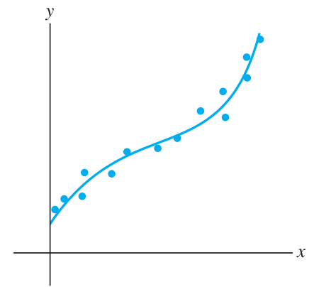
Finding a best fit cubic

Suppose we have some data like this:

Input:	1	2	3	4	5	6
Output:	5	9	8	4	6	8
Let’s fit a cubic polynomial to this data. We use the objects:

First, compute:

Row reduction of the augmented matrix yields:

Therefore our best fit cubic polynomial is:

Linear after some transformation

Some functions appear not to be amenable to linear regression, but they can be transformed to become so.

Consider the class of functions with two parameters and . These functions are not ‘summation curves’.

However, if we take the log of the observation vector, we can fit a linear function with parameters and :

LLS can be used to find the best fit values of and as if these are the -intercept and slope of a line. Taking reveals the desired from the discovered , and then and can be plugged back into .

Multiple regression

It frequently happens that our model predicts observations on the basis of multiple input variables. This situation can be handled using LLS in the same way as ‘summation curves’ are handled. The entries in the design matrix include all the input values, and the parameter vector provides the candidate coefficients for the linear combinations of those input values.

The design matrix will contain the values of and (for ) and , , , , and (for ) that correspond to the various output values in the observation vector. The parameter vector will be (for ) and (for ).

The graph of , given by setting , will be a plane passing through at . We can use LLS to find the plane of best fit for a collection of D vectors. For example, if we are given a set of points in D space:

then we can find the best fit plane by solving the following LLS problem:

Penrose quasi-inverse

The Penrose quasi-inverse, also called Moore-Penrose pseudo-inverse, is a matrix construction that always exists, and is very easy to find using the SVD, and it is directly related to the LLS problem.

Given a matrix , its Penrose quasi-inverse is the matrix . Here is derived from by first transposing, and second inverting the main diagonal entries (i.e. taking their reciprocals).

The meaning of this matrix is that it acts like an inverse for vectors in the image of , while for other vectors it first projects to and then applies the inversion after that.

The connection to LLS is that if and are given, then is the least-squares solution vector .

Which LLS solution is it?

If there are many solutions for , because has non-trivial null space, then, as you can see from the SVD formula, this picks the one with zero component in the kernel and nonzero part only in the cokernel. (This is the part spanned by the first vectors , up to the point where for .)

To summarize: LLS can have many solutions, but the single choice is the specific solution lying entirely in the cokernel of . Other solutions deviate by a difference vector which lies in the kernel of .

Example

Using Penrose quasi-inverse to solve LLS

In Packet 13 we found the following SVD:

Problem: Use the SVD above in order to (a) find the Penrose quasi-inverse , and (b) find a vector that minimizes for .

Solution: The quasi-inverse is formed by transposing and inverting the entries. We obtain for (a):

Then (b) to solve the LLS, we simply compute and obtain .

Notice that after calculating once, we can solve any LLS problem very efficiently. That is a nice feature.

Problems due 26 Apr 2024 by 11:59pm

Problem 14-01

Linear least-squares: non-orthogonal columns

Solve the linear least-squares problem for the following inconsistent system: Compute the error to two decimal places.

Problem 14-02

Linear least-squares: orthogonal columns

Solve the linear least-squares problem for the following inconsistent system, using the fact that the columns of are orthogonal: Compute the error to two decimal places.

Problem 14-03

Fitting a plane to four points

Consider the four data points in D space:

Find the parameters for which the plane defined by best fits these data points.

You may notice that the data points correspond to heights at the four corners of a square. Normally a plane is defined by 3 points (non-colinear) through which it passes. No plane passes through these four given points. But there is a plane that minimizes the sum of squares of vertical errors.

Problem 14-04

LLS summation curve model

Consider the data points: . Find the parameters of best fit for the model . Clearly identify your design matrix, observation vector, and parameter vector. Compute the error vector and the total error.

Problem 14-05

Penrose quasi-inverse

For this problem, use the definition of based on the SVD of .

• (a) Verify that and that for the example studied in the section on quasi-inverse. Think about how and why this happens in terms of the SVD.
• (b) Show that for any matrix, is the projection of onto the image of .
• (c) Show that for any matrix, and .

It may be helpful (though not required) for this problem to use the presentation of SVD in the form as in Packet 13. In order to use this, figure out what the corresponding presentation of the SVD of should be.

Problem 14-06

LLS uniqueness

• (a) Show that: if and only if . (Hint: use the fact that .)
• (b) Show that: is invertible if and only if has independent columns. (Warning: need not be square. Hint: consider the dimensions of kernels, and use (a) as well as the rank-nullity theorem.)
• (c) Explain why the LLS problem for and has a unique solution if and only if the columns of are independent. (Use (b).)
• (d) Continuing from (b), show that: . (Hint: apply rank-nullity to both matrices. Notice that and have the same number of columns.)

You may observe that (a) implies , while (d) means . In other words, and always have the same size kernels and the same size images. This makes sense in terms of the SVD if you think about kernels, cokernels, and images generated by the orthonormal basis vectors ’s and ’s, writing as in the previous problem (keeping careful track of which ’s are zero or nonzero!).