Applied Linear Algebra - Packet 15

Packet 15

Application II: Principal component analysis

Raw data points are row vectors. Each entry in the row corresponds to a variable. For example ${𝐚}^1=\left(\begin{array}{ccccc}\text{height}& \text{weight}& \text{age}& \text{BP}& \text{HR}\end{array}\right)$.

Defining PCA

For applications to dimension reduction, this row vector could be very large: $\mathrm{1,000}\times \mathrm{1,000}=1\text{M}$ pixel grayscale values: a single row with $1\text{M}$ entries.

Data matrix $A_0=\left(\begin{array}{ccc}-& {𝐚}^1& -\\ -& {𝐚}^2& -\\ ⋮& ⋮& ⋮\\ -& {𝐚}^n& -\end{array}\right)$ has row vectors that are data points. Each row is another data point. So $A_0$ is an $n\times m$ vector when the data lives in ${ℝ}^m$ and we have $n$ samples.

Sometimes $A$, sometimes $A^{𝖳}$

Some authors (e.g. Wikipedia and this Packet) put data points as row vectors. Others (Lay et al., Strang) put data points as column vectors. Pay attention.

Convert raw data $A_0$ to mean-deviation form:

$$A=A_0-\left(\begin{array}{cccc}{\mu }_1& {\mu }_2& \cdots & {\mu }_m\\ {\mu }_1& {\mu }_2& \cdots & {\mu }_m\\ ⋮& ⋮& \cdots & ⋮\\ {\mu }_1& {\mu }_2& \cdots & {\mu }_m\end{array}\right)$$

where ${\mu }_i$ is the average value of the entries in column $i$ of $A$. The entries of $A$ record the displacements of the entries of $A_0$ from the mean across all samples (per vector component of data vectors).

Compute the sample covariance matrix:

$$S=\frac{1}{n-1}{A}^{𝖳}A.$$

This is a symmetric $m\times m$ matrix. (Sized by # variables, not # samples.) The matrix $S$ is large when the row vectors are long, as for pixel data of images.

The division by $n-1$ comes from rule for calculating the covariance. (For more details, take a course in probability or statistics.)

The $(ij)$-entry of $S$ is the dot product ${𝐚}_i\cdot {𝐚}_j$. This dot product computes the covariance of variable $i$ and variable $j$ across the samples. The scale of this number depends on the number of samples and the relative scale of the typical variable values. After diving by $n-1$, it depends only on the typical variable values.

The matrix $S$ is symmetric so the spectral theorem applies. The eigenvalues of $S$ in order, ${\lambda }_1\ge {\lambda }_2\ge {\lambda }_3\ge \cdots$, are the principal variances of the data. The corresponding basis of (orthonormal) eigenvectors of $S$, namely ${𝐯}_1,{𝐯}_2,{𝐯}_3,\dots$, are the principal components of the data. The square roots ${\sigma }_1=\sqrt{{\lambda }_1},{\sigma }_2=\sqrt{{\lambda }_2},{\sigma }_3=\sqrt{{\lambda }_3},\dots$ may be called the principal deviations, although that term is not commonly used. In our notation where data vectors are rows of $A$, it is best to transpose the principal components into row vectors ${𝐯}_1,{𝐯}_2,{𝐯}_3,\dots$ that correspond to the format of the data vectors.

Discussion

The SVD of $A$ is implicit in the above. PCA is almost directly the SVD, but there are two formatting changes to watch out for.

• $A^{𝖳}$ may be used instead of $A$
• Factor of $\frac{1}{n-1}$ appearing on the symmetric matrix $S$

PCA ‘basically’ from SVD

PCA is derived from the SVD of $\frac{1}{\sqrt{n-1}}A$ (this Packet) or from $\frac{1}{n-1}{A}^{𝖳}$ (some authors).

If the data vectors are rows of $A$ and the variables are columns, then the right singular vectors of $\frac{1}{\sqrt{n-1}}A$ form the principal components, and singular values of this matrix form the principal variances.

If we already have the SVD, namely $A=U\mathrm{\Sigma }{V}^{𝖳}$, then ${\sigma }_i/\sqrt{n-1}$ are the principal variances, and ${𝐯}_i$ are the principal components.

For authors who write their data points as column vectors in the data matrix, the SVD of $\frac{1}{\sqrt{n-1}}{A}^{𝖳}$ gives the PCA data: singular values are principal variances, and left singular vectors are the principal components.

Some further terminology.

Statisticians like the concept of a variable. This concept meshes with probability theory as well. The variables are represented as the quantities in the entries of the rows ${𝐚}^i$ of the data matrix $A_0$. The entries of ${𝐯}_i^{𝖳}$ are also the values of variables.

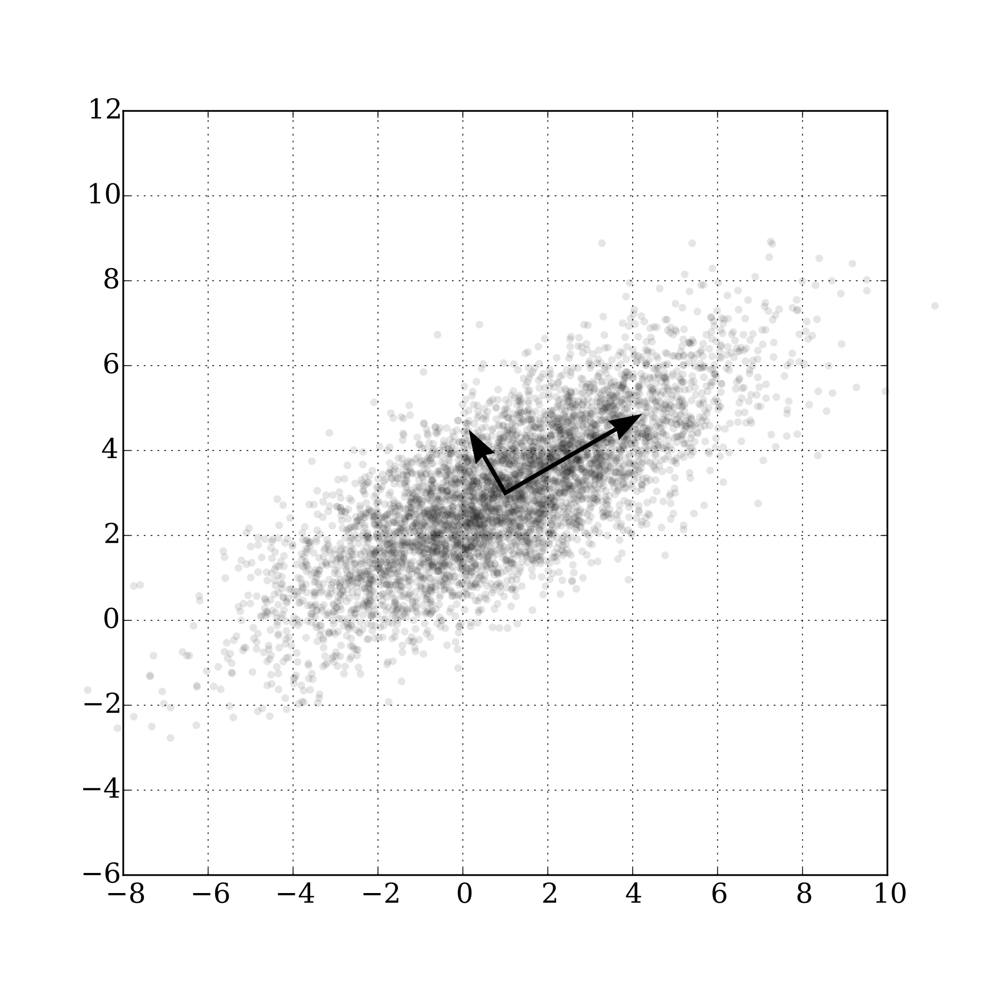
The vector ${𝐯}_1^{𝖳}$ is a unit vector pointing in the direction (in the data vector space) of the greatest variation in the data. The vector ${𝐯}_2^{𝖳}$ is a unit vector pointing in the direction (in the data vector space) of the greatest variation in the data from those directions that are orthogonal to ${𝐯}_1^{𝖳}$.

Suppose we take a variable (indeterminant) input vector $𝐗=\left(\begin{array}{cccc}{x}_1& x_2& \cdots & x_m\end{array}\right)$ in the data space. Suppose ${𝐯}_1^{𝖳}=\left(\begin{array}{cccc}{c}_1& c_2& \cdots & c_m\end{array}\right)$. Then the dot product

$$y_1=c_1{x}_1+c_2{x}_2+\cdots +c_m{x}_m$$

gives a new variable that corresponds to the first principal component. Variables for the remaining principal components can be given as well. Collecting all variables of the principal components:

$$𝐘=𝐗V.$$

• Variance of $𝐘=𝐗𝐯$ where $𝐗$ ranges across the data is as large as possible when $𝐯={𝐯}_1$ the first principal component.
• Variance capture percentage: ${\sigma }_i^2/({\sigma }_1^2+\cdots +{\sigma }_m^2)={\sigma }_i^2/\mathrm{tr}(S)$.

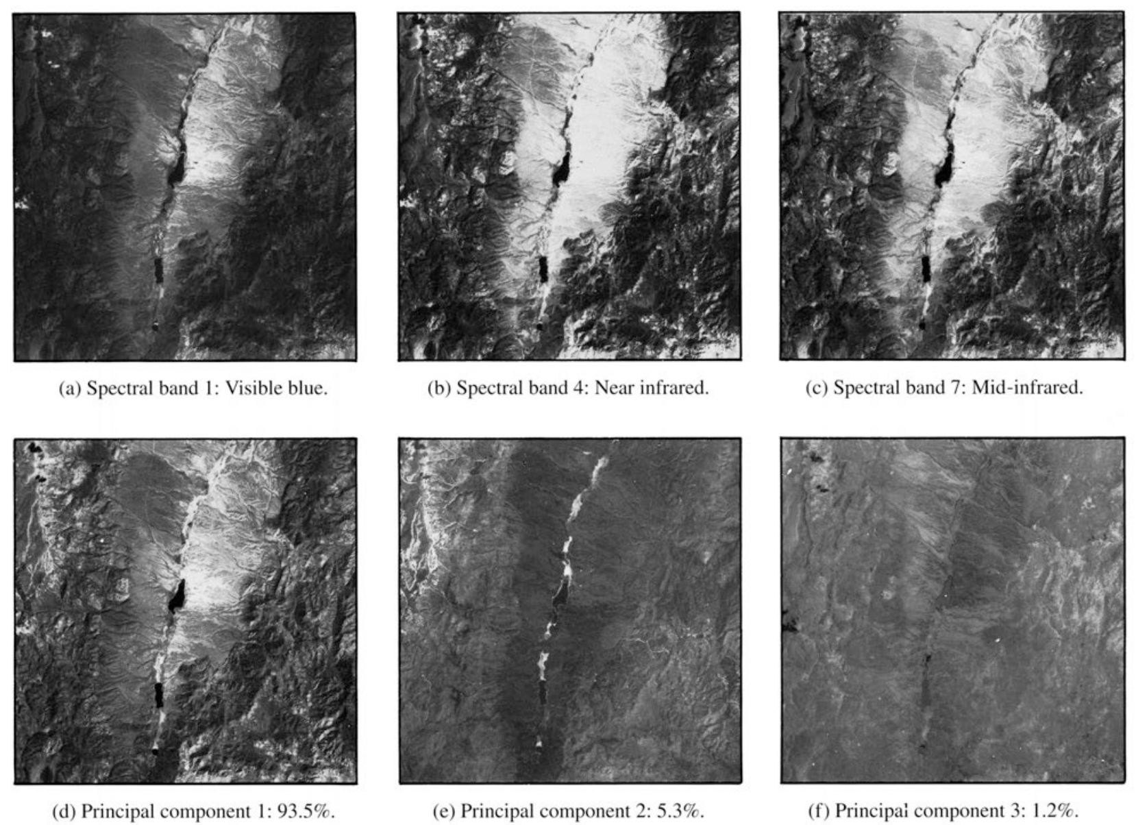
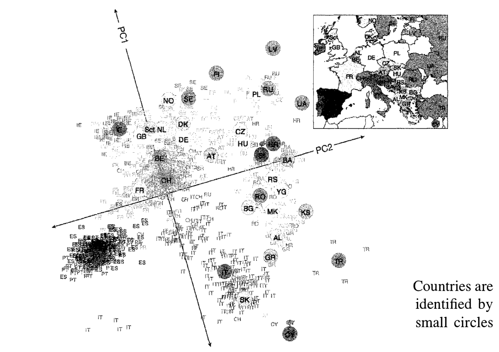
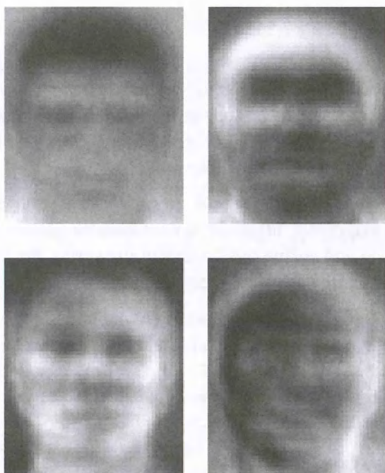
Applications of PCA