Power series as functions
Videos, Math Dr. Bob
- Power series functions: Derivative/Antiderivative - Basics
- Power series functions: Derivative/Antiderivative - Interval of Convergence
- Power series functions: Derivative/Antiderivative - More examples
- Power series functions: Geometric Power Series
01 Theory
Given a numerical value for
Many techniques from algebra and calculus can be applied to such power series functions.
Addition and Subtraction:
Summation notation:
Scaling:
Summation notation:
Extra - Multiplication and composition
Multiplication:
For example, suppose that the geometric power series
converges, so . Then we have for its square: Composition:
Assume:
Then:
Differentiation:
Antidifferentiation:
For example, for the geometric series we have:
Do the series created with sums, products, derivatives etc., all converge? On what interval?
For the algebraic operations, the resulting power series will converge wherever both of the original series converge.
For calculus operations, the radius is preserved, but the endpoints are not necessarily:
Power series calculus - Radius preserved
If the power series
has radius of convergence , then the power series and also have the same radius of convergence .
Power series calculus - Endpoints not preserved
It is possible that a power series
converges at and endpoint of its interval of convergence, yet and do not converge at .
Extra - Proof of radius for derivative and integral series
Suppose
has radius of convergence : Consider now the derivative
and its ratios of successive terms: Consider instead the antiderivative
and its ratios of successive terms: In both these cases the ratio test provides that the series converges when
.
02 Illustration
Example - Geometric series: algebra meets calculus
Geometric series: algebra meets calculus
Consider the geometric series as a power series functions:
Take the derivative of both sides of the function:
This means
satisfies the identity: Now compute the derivative of the series:
On the other hand, compute the square of the series:
So we find that the same relationship holds, namely
Link to original, for the closed formula and the series formula for this function.
Example - Manipulating geometric series: algebra
Manipulating geometric series: algebra
Find power series that represent the following functions:
(a)
(b) (c) (d) Solution
(a)
Rewrite in format
. Introduce double negative:
Choose
.
Plug
into geometric series. Geometric series in
: Plug in
: Simplify:
Final answer:
(b)
Rewrite in format
. Rewrite:
Choose
.
Plug
into geometric series. Geometric series in
: Plug in
: Final answer:
(c)
Rewrite in format
. Rewrite:
Choose
. Here .
Plug
into geometric series. Geometric series in
: Plug in
: Obtain:
Multiply by
. Distribute:
Final answer:
(d)
Rewrite in format
. Rewrite:
Choose
. Here .
Plug
into geometric series. Geometric series in
: Plug in
: Obtain:
Multiply by
. Distribute:
Final answer:
Link to original
Example - Manipulating geometric series: calculus
Manipulating geometric series: calculus
Find a power series that represents
. Solution
Differentiate to obtain similarity to geometric sum formula.
Differentiate
:
Find power series of differentiated function.
Power series by modifying
with :
Integrate series to find original function.
Integrate both sides:
Use known point to solve for
: Final answer:
Link to original
Example - Recognizing and manipulating geometric series: Part I
Recognizing and manipulating geometric series: Part I
(a) Evaluate
. (Hint: consider the series of .) (b) Find a series approximation for
. Solution
(a) Evaluate
. (Hint: consider the series of .) Find the series representation of
following the hint. Notice that
. We know the series of
: Notice that
; this is the desired function when . Integrate the series term-by-term:
Solve for
using , so and thus . So:
Notice the similar formula.
The series formula
looks similar to the formula .
Choose
to recreate the desired series. We obtain equality by setting
because . Final answer is
. (b) Find a series approximation for
. Observe that
. Therefore we can use the series
Plug
into the series for . Plug in and simplify: Link to original
Example - Recognizing and manipulating geometric series: Part II
Recognizing and manipulating geometric series: Part II
(a) Find a series representing
using differentiation. (b) Find a series representing
. Solution
(a) Find a series representing
. Notice that
. Obtain the series for
. Let
:
Integrate the series for
by terms. Set up the strategy. We know:
and:
Integrate term-by-term:
Conclude that:
Solve for
by testing at . Plugging in, obtain:
so
. Final answer is
. (b) Find a series representing
. Find a series representing the integrand.
Integrand is
. Rewrite integrand in format of geometric series sum:
Write the series:
Integrate the integrand series by terms.
Integrate term-by-term:
This is our final answer.
Link to original
Taylor and Maclaurin series
Videos, Math Dr. Bob
03 Theory
Suppose that we have a power series function:
Consider the successive derivatives of
When these functions are evaluated at
This last formula is the basis for Taylor and Maclaurin series:
Power series: Derivative-Coefficient Identity
This identity holds for a power series function
which has a nonzero radius of convergence.
We can apply the identity in both directions:
- Know
? Calculate for any . - Know
? Calculate for any .
Many functions can be ‘expressed’ or ‘represented’ near
Such a power series representation is called a Taylor series.
When
One power series representation we have already studied:
Whenever a function has a power series (Taylor or Maclaurin), the Derivative-Coefficient Identity may be applied to calculate the coefficients of that series.
Conversely, sometimes a series can be interpreted as an evaluated power series coming from
04 Illustration
Example - Maclaurin series of
Maclaurin series of e to the x
What is the Maclaurin series of
? Solution Because
, we find that for all . So
for all . Therefore for all by the Derivative-Coefficient identity. Thus:
Link to original
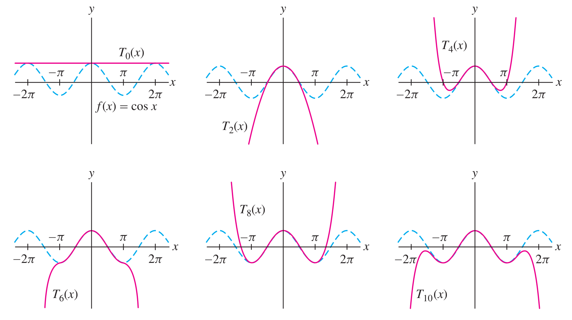
Example - Maclaurin series of
Maclaurin series of cos x
Find the Maclaurin series representation of
. Solution Use the Derivative-Coefficient Identity to solve for the coefficients:
0 1 2 3 4 5 By studying the generating pattern of the coefficients, we find for the series:
Link to original
Maclaurin series from other Maclaurin series
Maclaurin series from other Maclaurin series
(a) Find the Maclaurin series of
using the Maclaurin series of . (b) Find the Maclaurin series of
using the Maclaurin series of . (c) Using (b), find the value of
. Solution
(a)
Remember that
Differentiate
Differentiate term-by-term:
Take negative because
: Final answer is
(b)
Recall the series
Compute the series for
. Set
:
Compute the product.
Product of series:
(c)
Derivatives at
are calculable from series coefficients. Suppose we know the series
Then
. It may be easier to compute
for a given than to compute the derivative functions and then evaluate them.
Compute
. Write the series such that it reveals the coefficients:
Coefficient with
corresponds to the term with , not necessarily the term (e.g. if the first term is as here). Compute
:
Compute
. Use Derivative-Coefficient Identity:
Link to original
Computing a Taylor series
Computing a Taylor series
Find the first five terms of the Taylor series of
centered at . Solution A Taylor series is just a Maclaurin series that isn’t centered at
. The general format looks like this:
The coefficients satisfy
. (Notice the .) We find the coefficients by computing the derivatives and evaluating at
: By dividing by
we can write out the first terms of the series: Link to original
05 Theory
Study these!
- Memorize all of these series!
- Recognize all of these series!
- Recognize all of these summation formulas!
Applications of Taylor series
Videos, Math Dr. Bob
- Approximating with Maclaurin polynomials:
to find - Approximating with Taylor polynomials:
at to find
06 Theory reminder
Linear approximation is the technique of approximating a specific value of a function, say
Computing a linear approximation
For example, to approximate the value of
, set , set and , and set so . Then compute:
So . Finally:
Now recall the linearization of a function, which is itself another function:
Given a function
The graph of this linearization
The linearization
Computing a linearization
We set
, and we let . We compute
, and so . Plug everything in to find
: Now approximate
:
07 Theory
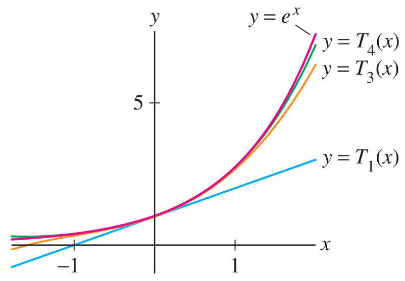
Taylor polynomials
The Taylor polynomials
of a function are the partial sums of the Taylor series of :
These polynomials are generalizations of linearization.
Specifically,
The Taylor series
Facts about Taylor series
The series
has the same derivatives as at the point . This fact can be verified by visual inspection of the series: apply the power rule and chain rule, then plug in and all factors left with will become zero. The difference
vanishes to order at : The factor
drives the whole function to zero with order as . If we only considered orders up to
, we might say that and are the same near .
08 Illustration
Taylor polynomial approximations
Taylor polynomial approximations
Let
and let be the Taylor polynomials expanded around . By considering the alternating series error bound, find the first
for which must have error less than . Solution
Write the Maclaurin series of
because we are expanding around . Alternating sign, odd function:
Notice this series is alternating, so AST error bound formula applies.
AST error bound formula is:
Here the series is
and is the error. Notice that
is part of the terms in this formula.
Implement error bound to set up equation for
. Find
such that , and therefore by the AST error bound formula: Plug in
. From the series of
we obtain for : We seek the first time it happens that
.
Solve for the first time
. Equations to solve:
Method: list the values:
The first time
is below happens when .
Interpret result and state the answer.
When
, the term at is less than . Therefore the sum of prior terms is accurate to an error of less than
. The sum of prior terms equals
. Since
because there is no term, the same sum is . The final answer is
. Link to originalIt would be wrong to infer at the beginning that the answer is
, or to solve to get .
Taylor polynomials to approximate a definite integral
Taylor polynomials to approximate a definite integral
Approximate
using a Taylor polynomial with an error no greater than . Solution
Write the series of the integrand.
Plug
into the series of :
Compute definite integral by terms.
Antiderivative by terms:
Plug in bounds for definite integral:
Notice AST, apply error formula.
Compute some terms:
So we can guarantee an error less than
by summing the first terms through . Final answer is
Link to original.