Polar curves
Videos, Organic Chemistry Tutor
01 Theory - Polar points, polar curves
Polar coordinates are pairs of numbers
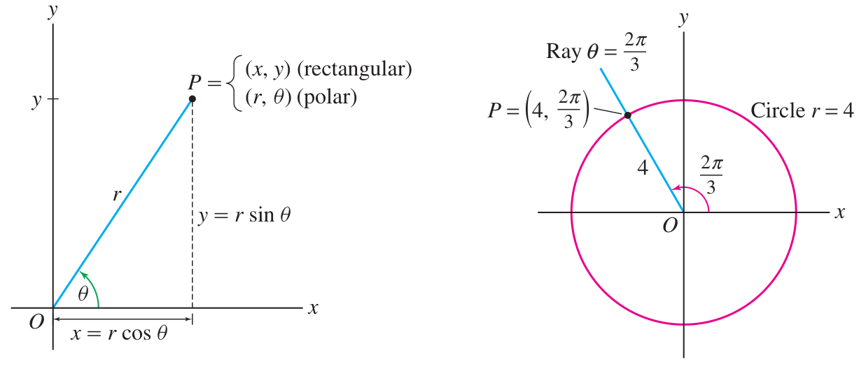
Converting
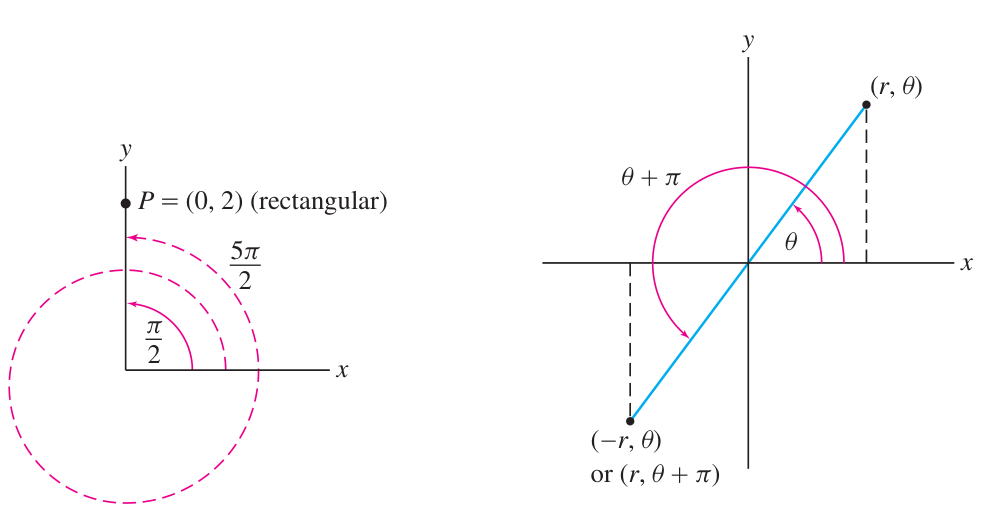
Polar coordinates have many redundancies: unlike Cartesian which are unique!
- For example:
- And therefore also
(negative can happen)
- And therefore also
- For example:
for every - For example:
for any
Polar coordinates cannot be added: they are not vector components!
- For example
- Whereas Cartesian coordinates can be added:
The transition formulas
require careful choice of .
- The standard definition of
sometimes gives wrong
- This is because it uses the restricted domain
; the polar interpretation is: only points in Quadrant I and Quadrant IV (SAFE QUADRANTS) - Therefore: check signs of
and to see which quadrant, maybe need -correction!
- Quadrant I or IV: polar angle is
polar angle is
Equations (as well as points) can also be converted to polar.
For
For
- For example:
02 Illustration
Converting to polar:
-correction Converting to polar: pi-correction
Compute the polar coordinates of
and of . Solution
For
we observe first that it lies in Quadrant II. Next compute:
This angle is in Quadrant IV. We add
to get the polar angle in Quadrant II: The radius is of course
since this point lies on the unit circle. Therefore polar coordinates are . For
we observe first that it lies in Quadrant IV. (No extra needed.) Next compute:
So the point in polar is
Link to original.
Shifted circle in polar
Shifted circle in polar
For example, let’s convert a shifted circle to polar. Say we have the Cartesian equation:
Then to find the polar we substitute
and and simplify: So this shifted circle is the polar graph of the polar function
Link to original.
03 Theory - Polar limaçons
To draw the polar graph of some function, it can help to first draw the Cartesian graph of the function. (In other words, set
This Cartesian graph may be called a graphing tool for the polar graph.
A limaçon is the polar graph of
Any limaçon shape can be obtained by adjusting
Limaçon satisfying
Limaçon satisfying
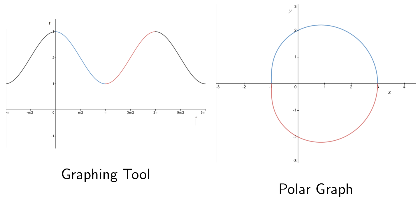
Limaçon satisfying
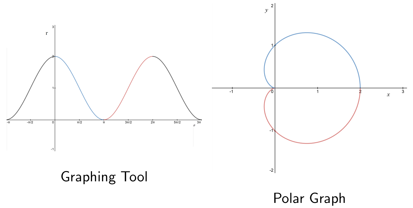
Limaçon satisfying
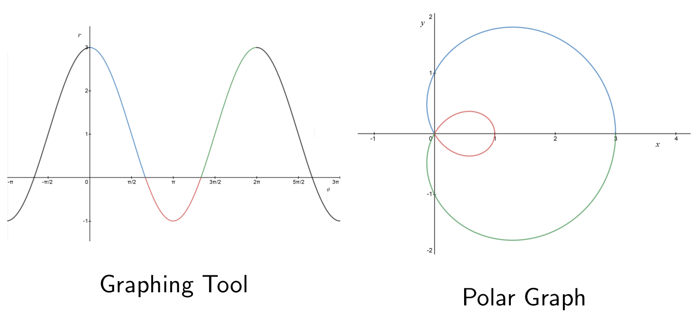
Limaçon satisfying
Limaçon satisfying
Transitions between limaçon types,
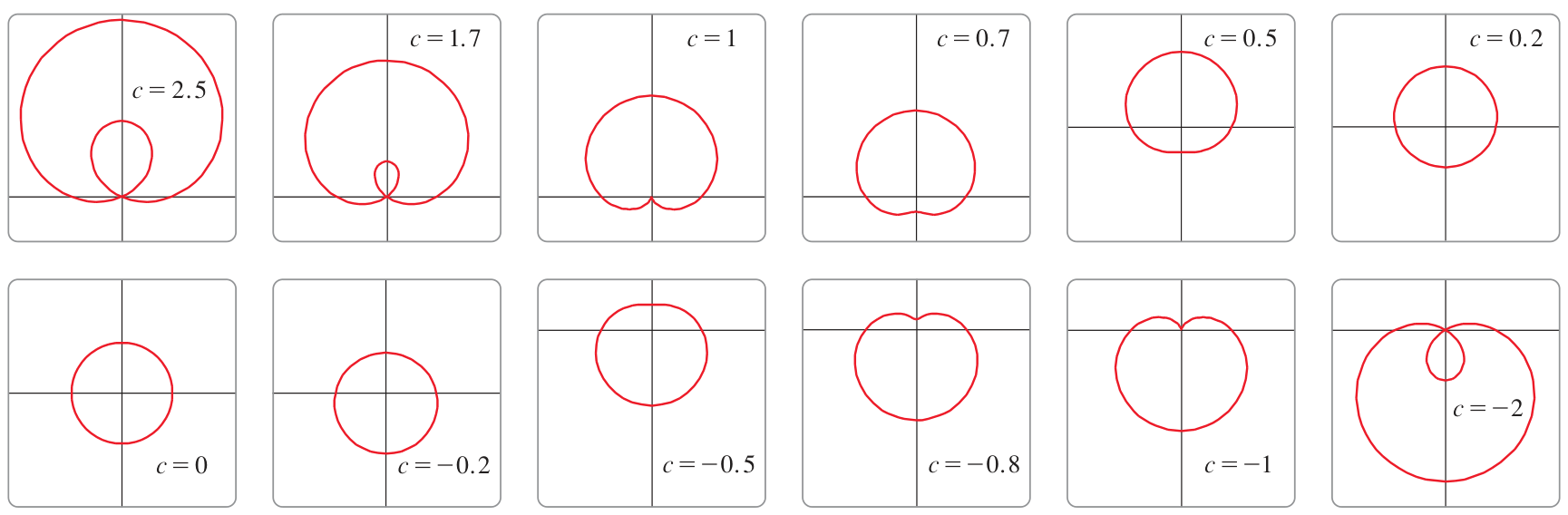
Notice the transition points at
The flat spot occurs when
- Smaller
gives convex shape
The cusp occurs when
- Smaller
gives dimple (assuming ) - Larger
gives inner loop
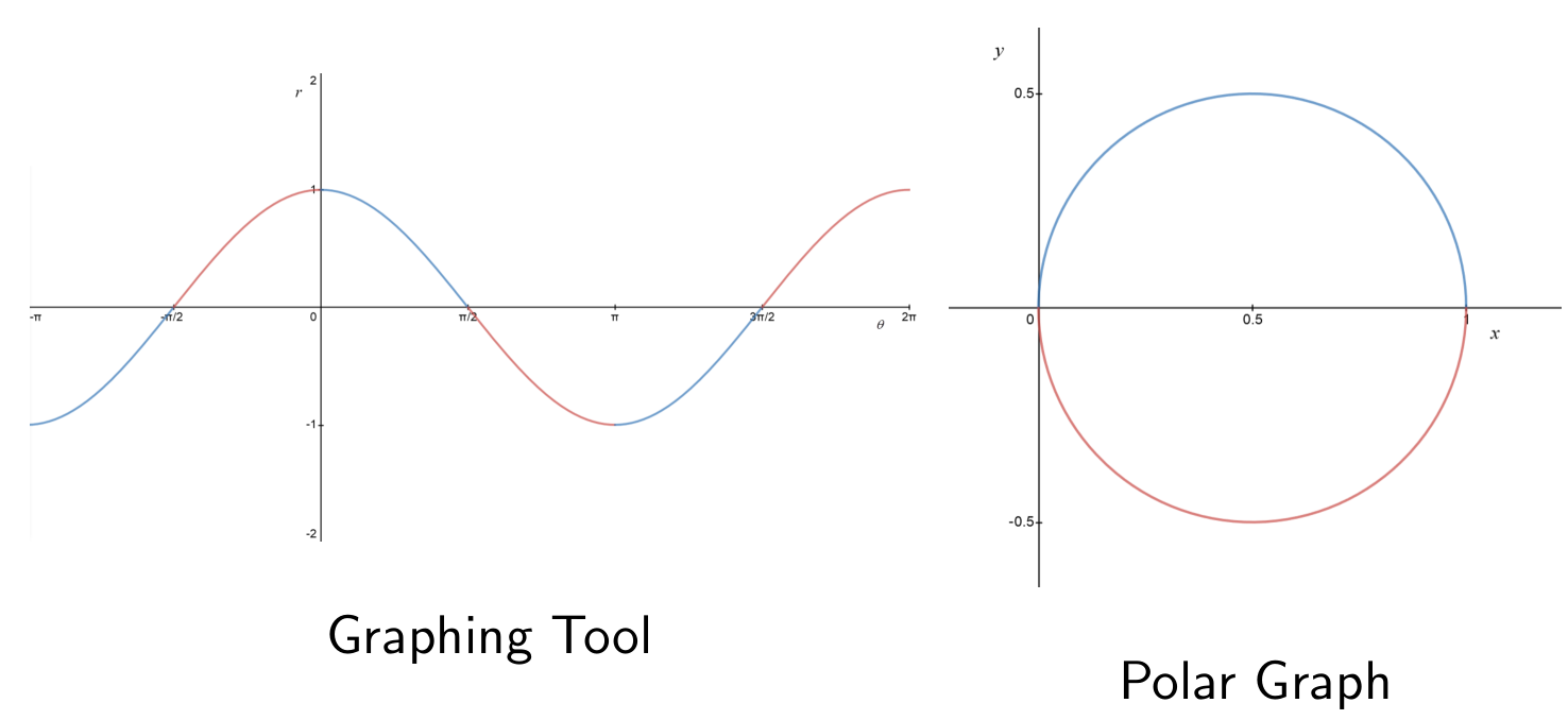
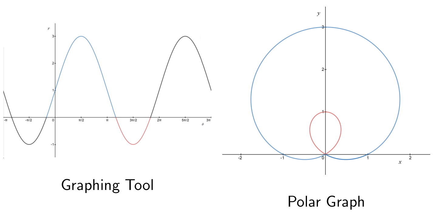
04 Theory - Polar roses
Roses are polar graphs of this form:
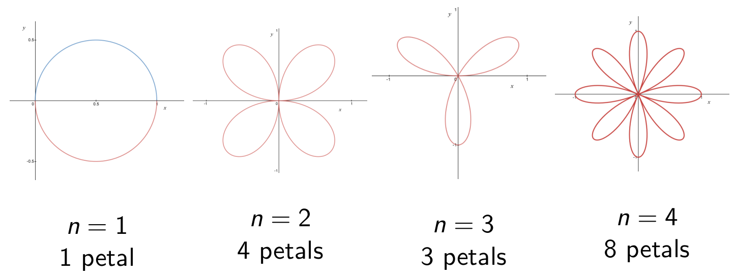
The pattern of petals:
(even): obtain petals - These petals traversed once
(odd): obtain petals - These petals traversed twice
- Either way: total-petal-traversals: always
Calculus with polar curves
05 Theory - Polar tangent lines, arclength
Polar arclength formula
The arclength of the polar graph of
, for :
To derive this formula, convert to Cartesian with parameter
From here you can apply the familiar arclength formula with
Extra - Derivation of polar arclength formula
Let
and convert to parametric Cartesian, so and . Then:
Therefore:
Therefore:
Therefore:
06 Illustration
Finding vertical tangents to a limaçon
Finding vertical tangents to a limaçon
Let us find the vertical tangents to the limaçon (the cardioid) given by
. Convert to Cartesian parametric.
Plug
into and :
Compute
and . Derivatives of both coordinates:
Simplify:
The vertical tangents occur when
. Set equation:
: Solve equation.
Convert to only
: Substitute
and simplify: Solve:
Solve for
:
Compute final points.
In polar coordinates, the final points are:
In Cartesian coordinates:
For
: For
: For
:
Correction:
is a cusp. The point
at is on the cardioid, but the curve is not smooth there, this is a cusp. Still, the left- and right-sided tangents exists and are equal, so in a sense we can still say the curve has vertical tangent at
Link to original.
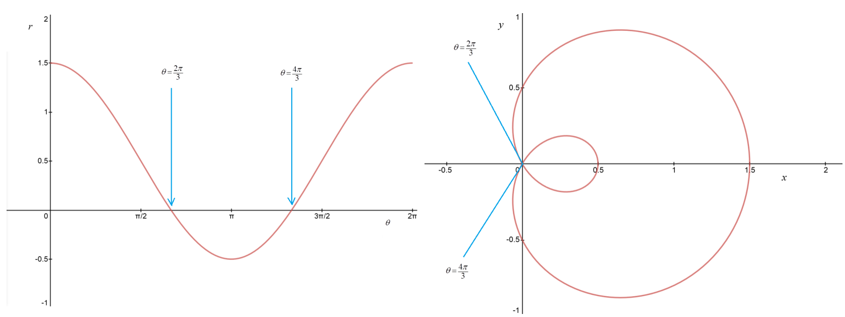
Length of the inner loop
Length of the inner loop
Consider the limaçon given by
. How long is its inner loop? Set up an integral for this quantity. Solution
The inner loop is traced by the moving point when
. This can be seen from the graph: Therefore the length of the inner loop is given by this integral:
Link to original
07 Theory - Polar area
Sectorial area from polar curve
The “area under the curve” concept for graphs of functions in Cartesian coordinates translates to a “sectorial area” concept for polar graphs. To compute this area using an integral, we divide the region into Riemann sums of small sector slices.
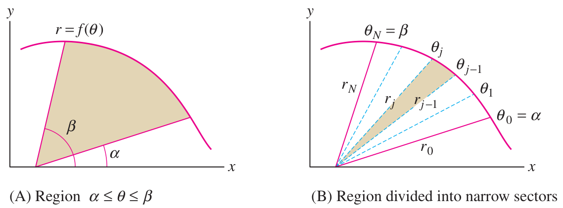
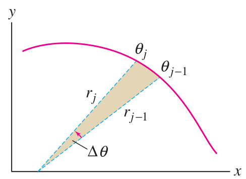
To obtain a formula for the whole area, we need a formula for the area of each sector slice.
Area of sector slice
Let us verify that the area of a sector slice is
.
Take the angle
in radians and divide by to get the fraction of the whole disk. Then multiply this fraction by
(whole disk area) to get the area of the sector slice.
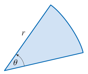
Now use
One easily verifies this formula for a circle.
Let
The sectorial area between curves:
Sectorial area between polar curves
Subtract after squaring, not before!
This aspect is not similar to the Cartesian version:
08 Illustration
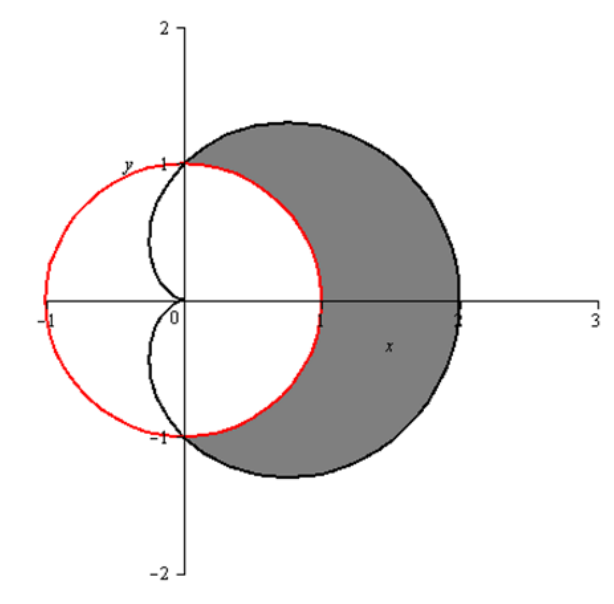
Area between circle and limaçon
Area between circle and limaçon
Find the area of the region enclosed between the circle
and the limaçon . Solution
First draw the region:
The two curves intersect at
. Therefore the area enclosed is given by integrating over : Link to original
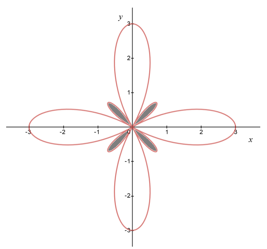
Area of small loops
Area of small loops
Consider the following polar graph of
: Find the area of the shaded region.
Solution
Bounds for one small loop.
Lower left loop occurs first.
This loop when
. Solve this:
Area integral.
Arrange and expand area integral:
Simplify integral using power-to-frequency:
with : Compute integral:
Link to original
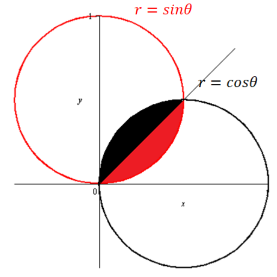
Overlap area of circles
Overlap area of circles
Compute the area of the overlap between crossing circles. For concreteness, suppose one of the circles is given by
and the other is given by . Solution
Here is a drawing of the overlap:
Notice: total overlap area =
area of red region. Bounds:
.
Apply area formula for the red region.
Area formula applied to
: Power-to-frequency:
: Double the result to include the black region:
Link to original