What are differential equations?
Examples of differential equations
The next examples illustrate what some important differential equations look like. Some other matters come up too, for example that solutions to differential equations are functions (not numbers), and that a single equation can have many solutions.
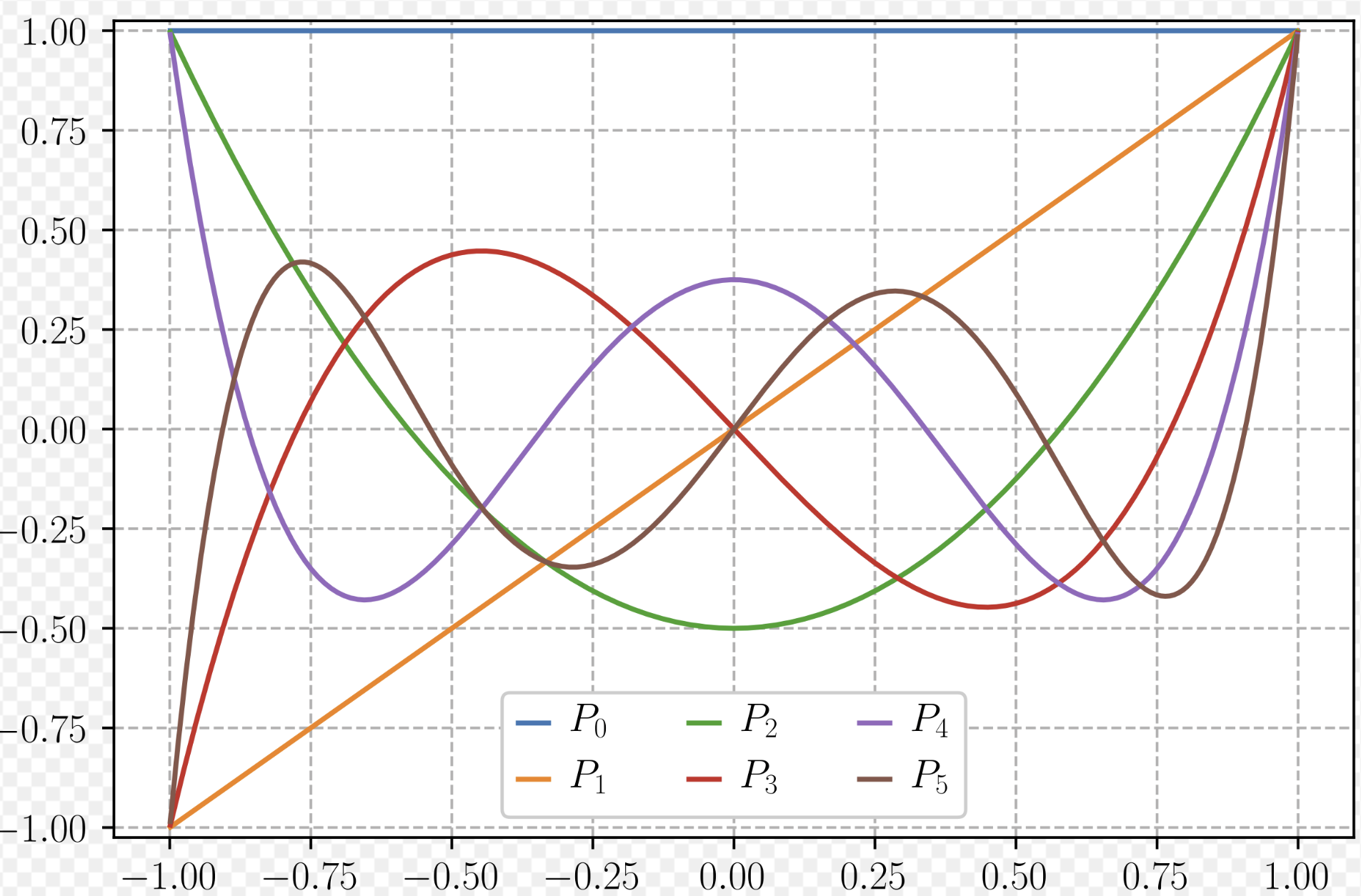
Legendre’s equation:
The solution to this equation is a polynomial for each . The first few polynomials are:
| 0 | 1 |
| 1 | |
| 2 | |
| 3 | |
| These polynomials have many useful properties. Their most important property is “orthogonality”: |
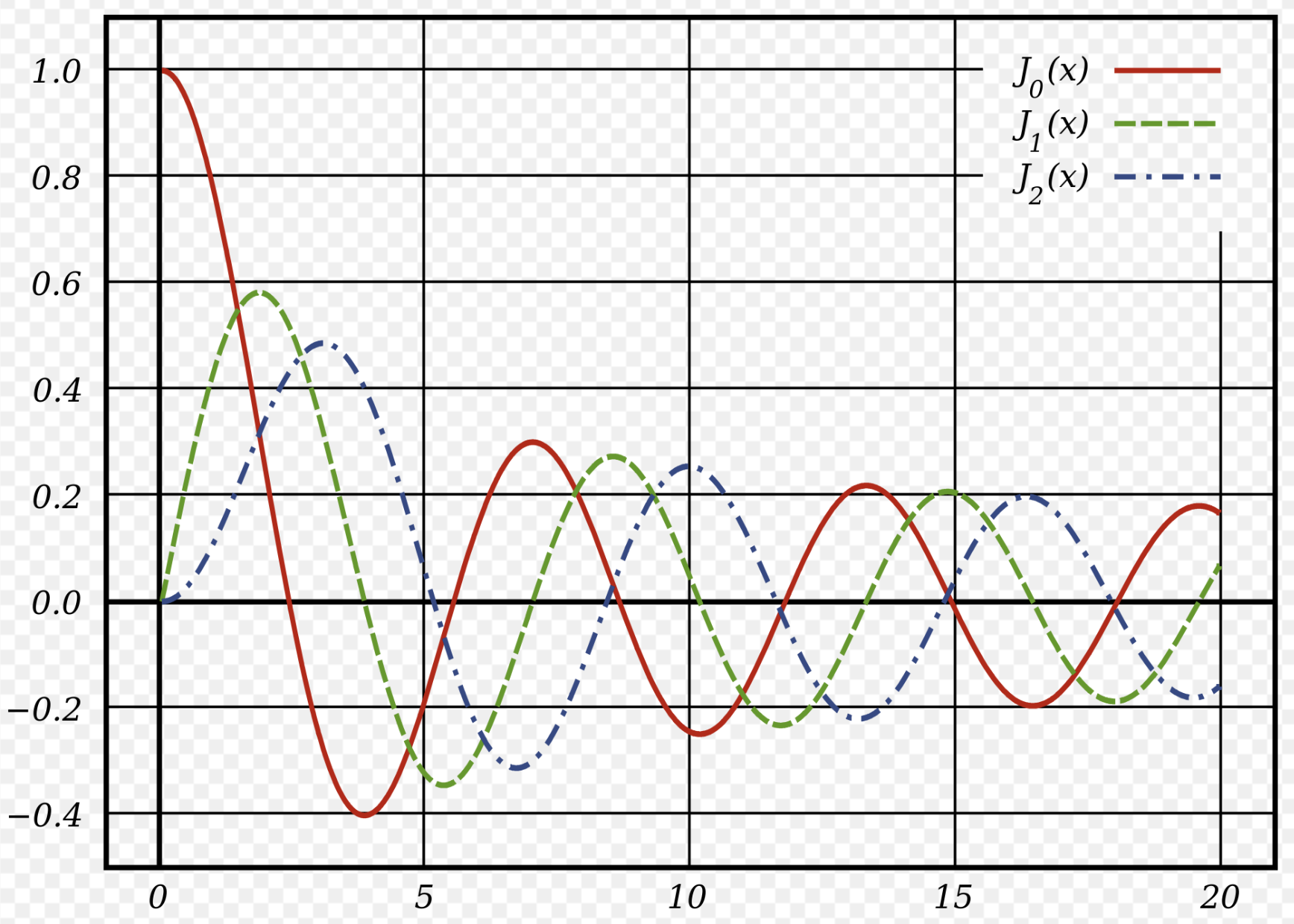
Bessel’s equation:
Solutions to this equation are used to study heat conduction and waves (electromagnetic or quantum wavefunctions).
Airy’s equation:
The solution to Airy’s equation arises in quantum mechanics, optics, and probability.
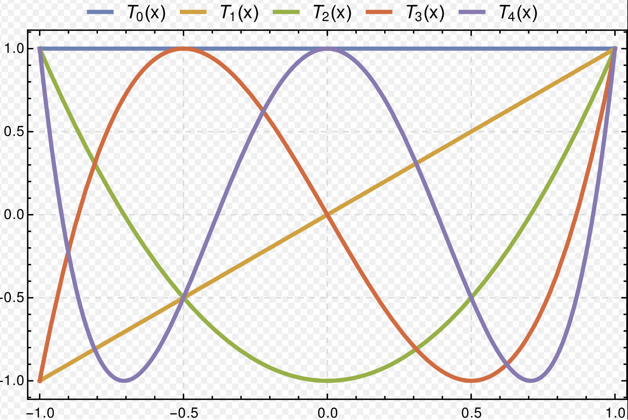
Chebyshev’s equation:
Solutions to this equation give polynomials and that describe the higher sum rules of trig functions:
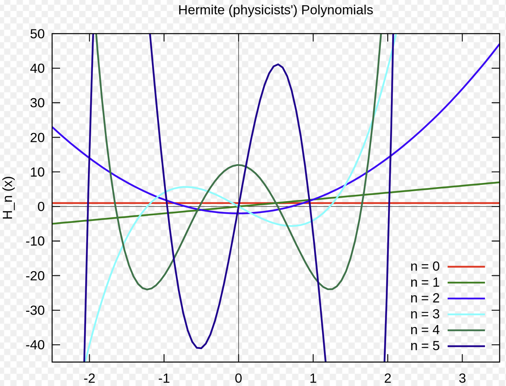
Hermite’s equation:
Solutions to this equation are used in quantum mechanics, signal processing, numerical analysis, and probability.
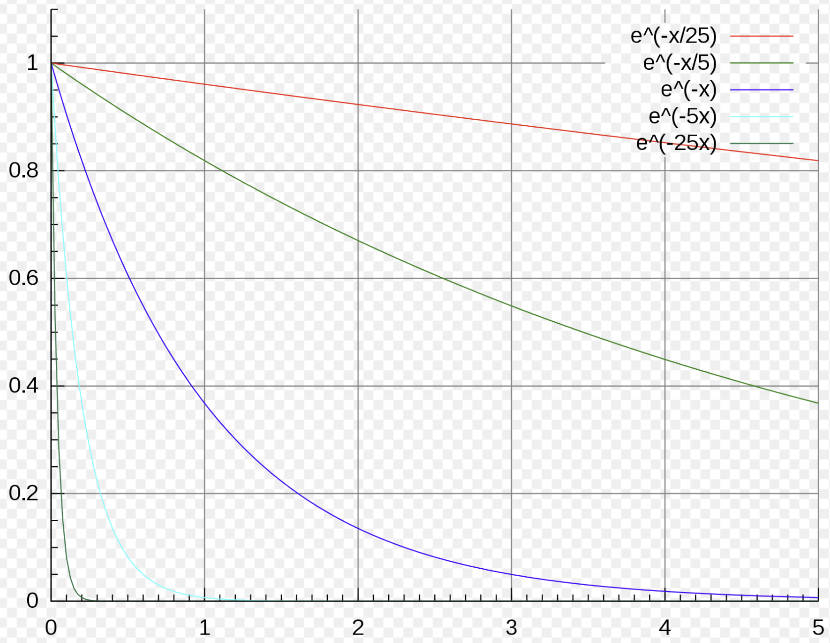
Exponential decay:
This equation models countless physical processes.
Concepts of differential equations
What we typically mean by a “differential equation” is a function of, say, variables, that is given by some algebraic expression (possibly involving trig or exponential functions as well). A solution to the equation is a function with the property that:
for all . The order of the differential equation is the order of the highest derivative that appears in the expression for .
A differential equation is called explicit when it can be written with the highest derivative isolated, on the other side:
Sometimes a differential equation is “solved” by finding an equation relating and which cannot be solved explicitly for in terms of . In this situation, a (connected) set of points satisfying the solution equation is called an integral curve of the differential equation.
Ordinary differential equations involve only ordinary derivatives, while partial differential equations involve partial derivatives.
Usually we assume that is a familiar kind of function that is constructed using algebraic operations (possibly with trig or exponential functions) applied to the arguments.
There is a fundamental distinction between linear and nonlinear differential equations. A linear differential operator is a linear function taking functions to functions. For example:
Question 02-01
Linear operator
Show that the example differential operator above satisfies the linearity equation for two given functions and . Let ; show that:
Linear differential equations are defined as those corresponding to a linear differential operator. (By applying the operator to and setting the result equal to some function.) Roughly speaking, this means they are equations in which can appear only to the first power.
First-order equations
A first-order (explicit) ODE looks like this:
for some function .
Many techniques for solving first-order ODEs come from reverse-engineering results of calculus. In this respect, solving ODEs analytically is like taking integrals (finding antiderivatives) analytically. In fact, antidifferentiation is itself one of the techniques: when does not depend on , both sides of the equation above can be integrated to find . More advanced methods like the product rule or -substitution yield more sophisticated techniques for ODEs.
Direct integration
A differential equation of the form:
has a set of solutions given by where is any constant and is an antiderivative of , meaning .
This kind of differential equation is really a part of basic calculus. A few things to emphasize en route to more complicated ODEs:
- There is a family of solutions parametrized by some constant . (This will become a pattern.)
- This family is a complete set: there are no other solutions. (Why not?)
- A particular solution is determined (selected from this family) by a choice of initial condition, which consists of a point that should lie on the solution.
- Consider that the derivative value specifies the direction of travel. So the initial condition is a starting point, and gives the data of which way to go, changing course along the route.
This technique can be applied in a series for simple ODEs of higher order. For example, the ODE
is solved by taking two antiderivatives. Let and . Then we have a family of solutions that depends on two constants:
To specify a particular solution, one provides two points and that should lie on the solution, and you can solve for and by evaluating and .
Question 02-03
Checking things
- For the first-order equation above, why must give a complete set of solutions?
- For the second-order equation, explain how to obtain the formula .
Question 02-04
Higher order
(Big Bonus question. Not for the faint of heart!)
- Can any two points and be chosen?
- Now iterate the process: consider and solve using multiple consecutive integrations. Describe the family of solutions. What constraints are there on the set of points needed to specify a particular solution?
Instead of providing multiple points lying on the solution, one can choose a single value , and then specify the values of the higher derivatives using some numbers .
Separable equations: substitution
Consider again the general form of an explicit first-order ODE:
This ODE is called separable when for some product of functions of the separate variables, and . It is solved by integrating separately in and in , as we consider next.
Consider any function with antiderivative , so . The chain rule says:
Now let . The differential equation
is equivalent to the equation
so we end up with
which is solved by integrating both sides in to obtain:
where is an antiderivative of and is a constant of integration.
Think about this equation . It equates the antiderivatives of and (up to a constant). It is an implicit definition of , because it may be virtually impossible to solve for here as a function of . And, for the same reason as used for the ODE earlier, the family of implicit curves given by this equation (for various ) describes all possible solutions.
Many authors describe the solution method a little differently. Starting with
write it as
and “integrate” both sides, summing up the differentials:
This yields
as before.
This method is easy to remember, and is acceptable to use on an exam or HW, but it is not really standard calculus procedure, since it relies on ambiguous rules about differentials. (Normally in calculus books differentials are considered purely mnemonic devices.)
Example
Separable ODE
Problem: Solve the equation . Solution: The given equation can be written
Integrating both sides, obtain
Applying on both sides:
Applying the exponent sum rule and writing , we get
Here because for any . However, we can allow by removing the absolute values. So that family of functions is the same as this family:
Note that the solution, , is valid but isn’t generated by separation of variables because of the division by that was performed in the first step.
Exercise 02A-01
Tricky signs
Check and explain all absolute values and signs (including ) in the previous example.
Example
Integral curves
Problem: Solve the separable ODE:
Solution: Rewrite this as:
and integrate both sides to obtain:
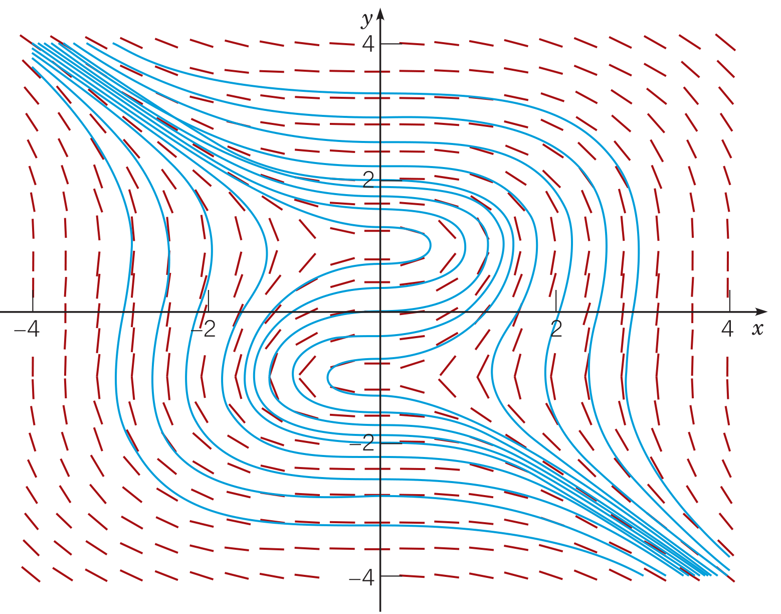
This equation specifies a family of integral curves. For the integral curves, we do not need to solve for in terms of . Here is a depiction:
Exercise 02A-02
Separable equations: basics
Solve the equations:
- (a)
- (b)
Exercise 02A-03
Separable equations: tricky trig
Solve the equation:
After finding the basic solution, check over the signs and absolute values of everything.
Exercise 02A-04
Particular solution
Find the particular solution to
which includes the point .
Linear equations: product rule
First-order linear equations have this general form:
These equations are solved using the product rule together with an “integrating factor” . It works like this. Apply the product rule to :
Now, multiply the original equation on both sides by to find:
Integrate both sides with respect to :
which can be solved for :
Example
First-order linear
Problem: Solve the equation:
Solution: First divide by to recover the standard format:
Now the integrating factor we need is . Multiply everything by this factor:
If everywhere, we can drop the absolute value signs obtaining . If everywhere, we would need to introduce minus signs (recall that and when ), obtaining ; but this we can multiply by and obtain the same equation, namely:
Let us solve this and come back later to consider the possibility of changing signs.
The sum on the left is the output of the product rule: . Now integrate in to find a family of solutions:
This family, for various values of , is our proposed solution to the ODE.
Now reconsider the absolute values. Suppose . If we take a solution curve with , then the entire curve will satisfy because as . Similarly, if we start with , then as . No solution crosses over . Now if we can say the same thing but with and , respectively, instead. Therefore our analysis using cases and is justified.
Exercise 02B-01
Linear equations: basics
Solve the following ODEs, giving a complete family of solutions:
- (a) ,
- (b) .
Exercise 02B-02
Linear equation: particular solution
Find a particular solution of the following ODE which passes through the point :
Exact equations: gradients
A final technique is based on more advanced calculus.
Recall the theorem of vector calculus:
Curl-free fields are gradients
Suppose is a vector field on with zero curl: . (Assume the region is simply-connected.) Then there is a scalar field whose gradient recovers the vector field: .
Writing out the components, this theorem says that if
then there is a function satisfying
Now, finally, let be a level curve given by for some . Then is perpendicular to . This latter fact can be interpreted as a differential equation with one of its integral curves, as we show next.
Let be considered a function of whose graph is the curve . Then may be described parametrically by , and the tangent vector to this parametric curve is described parametrically by . The condition is equivalent to , which when written out means:
Writing and and , and multiplying through by , we obtain a form that is easier to remember:
Here is a summary of our reasoning:
Exact equations
Suppose the differential equation written either in form (A):
or in form (B):
satisfies . Then it has a family of solutions given by the level curves , where is a function satisfying and .
Algebraic summary
A more algebraic formulation of the same theory goes like this:
If , then it is possible to find such that and . In this case the equation
can be written
using the chain rule, and this has as solutions the family of integral curves defined implicitly with constants :
Example
Solving an exact equation
Problem: Solve the ODE:
Solution: First we check that :
Now we seek with and . First integrate in :
where the “constant” can be any function of . Now , so and . Therefore our solution family of integral curves is given by:
for .
Exercise 02B-03
Checking exactness
Which of the following ODEs are exact?
- (a)
- (b)
- (c)
- (d)
Exercise 02B-04
Solving an exact equation
Show that the ODE is exact, and solve it:
Problems: due Monday 29 Jan 2024 by 1:00pm
Problem 02-01
Decide whether the ODE is separable, first-order linear, or exact, and then solve it:
- (a)
- (b)
- (c)
- (d)
- (e)
- (f)
Problem 02-02
Exact equation: 2D gradient emanating from charged particle
Consider an electric field in given by:
Find a scalar function whose gradient is . What are the level curves of ? Now write an exact differential equation whose integral curves are these level curves of .