Differential Equations - Packet 03

Transformation and reduction

So far we have seen how to solve differential equations by direct integration, by separation of variables, by integrating factors: conversion to a product (linear equations), and by gradients (exact equations).

Many differential equations do not immediately appear to have the standard form to which these methods are applicable, but in fact these methods can be applied after performing a transformation. The possibility of some of these transformations can be checked systematically, but for others we rely on an art – not a mechanical science – of finding an appropriate substitution. This art is based on experience and honed by practice.

Homogeneous equations: conversion to separable

Homogeneous functions A function is homogeneous when the input variable appears everywhere in the same degree. More precisely and technically, is homogeneous when for some . Similarly is homogeneous when for some . (Likewise for more variables.) In this situation is called the degree of homogeneity.

In other words, a function is homogeneous when the action of scaling the inputs simultaneously can be factored out to an action of scaling the output.

For example, these functions are homogeneous:

whereas these are not:

Homogeneous differential equations Now, suppose we have a differential equation in the form:

where and are homogeneous functions of the same degree. Then the change of variables (by substituting ) will convert the quotient on the right to a function of alone, and the equation as a whole to a separable equation, which we can solve for and at the end the solution can be converted to an expression in by substituting back .

Homogeneous substitution

Suppose and are homogeneous of the same degree . Then depends only on the ratio :

Separability then occurs because:

so the equation is equivalent to

and the general solution is the family of curves given by:

Alternate format The differential equation

is homogeneous if and are both homogeneous of the same degree. It can be transformed with the same substitution and the result is separable.

Question 03-01

Homogeneous?

Is a homogeneous differential equation?

Example

Homogeneous equation

Consider the differential equation . Assuming , this is equivalent to the homogeneous equation . Define , and we find:

The solution is therefore , or for any , i.e. .

Example

See an example in “Families of integral curves” below, where we solve the homogeneous equation .

Exercise 03A-01

Homogeneous equations

For the following differential equations, show that they are homogeneous, and then solve them by substitution and separation:

• (a)
• (b)
• (c)

Linear quotients: almost homogeneous Suppose we are given a differential equation

This equation is not homogeneous, but it is easily converted to a homogeneous equation by a change of variables. Find that solve the system:

Then by plugging in and , the quotient on the right side is transformed to a quotient of homogeneous functions in and :

The left side transforms as desired:

Question 03-02

Transform linear quotient to homogeneous

Transform this equation to a homogeneous equation:

Integrating factors: conversion to exact

Sometimes an equation

is not exact, but there is a function which when multiplied through the equation gives an exact equation:

Question 03-03

Integrating factor

Check that is an integrating factor for .

How can we find such a function ? There is no recipe that can find all possibilities for . However, if there is a that works and is a function of either or alone, then there is a recipe. Here it is:

Integrating factors: single variable

• Check : if the function depends on alone, we can use .
• Check : if the function depends on alone, we can use .

Exercise 03A-02

Method of integrating factors

Show that if the function depends on alone, we can use as an integrating factor and the resulting differential equation becomes exact.

Example

Integrating factor: converting to exact

Consider the differential equation . This is not exact because while . However, is a function of alone. Therefore we can use as an integrating factor. Multiplying through by produces the equation , which is exact because now .

Exercise 03A-03

Integrating factor: converting to exact

Convert the following to exact equations by finding and applying integrating factors.

• (a)
• (b)

Reduction of order

Some second-order ODEs can be reduced to first-order ODEs by substituting . This works when the equation is missing either or .

If the equation is missing , so the ODE is actually given by , then we substitute and , and try to solve the equation as any other first-order equation. Afterwards we can solve for by integrating (provided we have an explicit solution for ).

If the equation is missing , so the ODE is actually given by , then we substitute as before, but now we let depend on , and so by the chain rule:

We therefore try to solve the equation as any other first-order equation.

Question 03-04

Reduction of order

Reduce the order of the following two differential equations. (No need to solve them.)

• (a)
• (b)

Example

Reduction of order

Consider . This equation is missing so we can reduce it to a first-order equation by letting and . The equation becomes which is separable. The solution is , and this implies . (Integrating to obtain .)

Consider . This equation is missing so we can reduce it to a first-order equation by letting and . The equation becomes which is separable. The solution is . This is a new differential equation which is also separable. Its general solution is .

Ad hoc transformations

Bernoulli equations The Bernoulli equations look like linear equations but with an extra factor of :

If we substitute , a Bernoulli equation becomes a linear equation.

Exercise 03A-04

Bernoulli substitution

Show that substituting does indeed convert the Bernoulli equation to a linear equation.

Exercise 03A-05

Solving Bernoulli equations

Solve the Bernoulli equation .

Linear substitutions If in the general form of an explicit first-order equation the items and only occur together in a linear combination, so it really takes the form , then we can change variables using and then separate variables. First convert :

then the equation becomes , which is separable:

Swapping roles It is sometimes effective to transform an equation to a known form by swapping the roles of and , meaning that is to be treated as the dependent variable and as the independent. To do this we need to replace with . This can be explained and justified using the theory for derivatives of inverse functions.

Inverse functions derivatives

If , then so . Now treating , we have . Therefore .

Example

Swapping roles

Consider the differential equation . If we change to , the equation becomes

or or . (This is linear of the form .) To solve it we write and thus or .

Exercise 03A-06

Swapping roles

Reverse the roles of and to solve: .

Families of integral curves

Each first-order differential equation leads to a family of curves, its integral curves (solution curves).

Conversely, each family of curves given by a single equation with a single parameter leads to a differential equation, and it is the equation whose solution curves are given by this family.

This correspondence

works in general, assuming the family of curves is provided by an equation (without derivatives) with a single varying parameter.

Example

Family of curves

For example, start with the family given by . Differentiate both sides: . Now plug in from the original equation, and we get the differential equation:

Conversely, let us solve this differential equation. Write it as:

This is a homogeneous equation, so we can substitute :

Integrating both sides, applying , and substituting gives:

Now multiply the fraction by and cross multiply to obtain , which is equivalent to assuming . Allowing , we have the original equation.

Something interesting we can do is define the orthogonal family of curves to a given family of curves. The orthogonal family is the family such that each curve is perpendicular to every curve of the original family.

For example, if one family of curves represents electric field lines, its orthogonal family represents equipotential lines. Or, if one family represents the level curves of a function, its orthogonal family represents the lines of steepest ascent.

The orthogonal family can be found from the original family by first computing the differential equation . The orthogonal family will be given by the differential equation . (The orthogonal slope is the negative reciprocal slope.)

Example

Circles and rays

We verify that the family of rays emanating from the origin is the orthogonal family to the family of circles centered at the origin. The family of circles is given by . This corresponds to the differential equation . The orthogonal family is then given by . Separating variables: so and thus for . This is the family of rays.

Exercises B

Exercise 03B-01

Homogeneous

Solve the following homogeneous equations by substitution of . You should first write the equation using a single quotient and then divide above and below by .

• (a)
• (b)

Exercise 03B-02

Integrating factors, conversion to exact

Solve the following differential equations by finding an integrating factor or .

• (a)
• (b)

Exercise 03B-03

Bernoulli

Solve the following Bernoulli equation: .

Exercise 03B-04

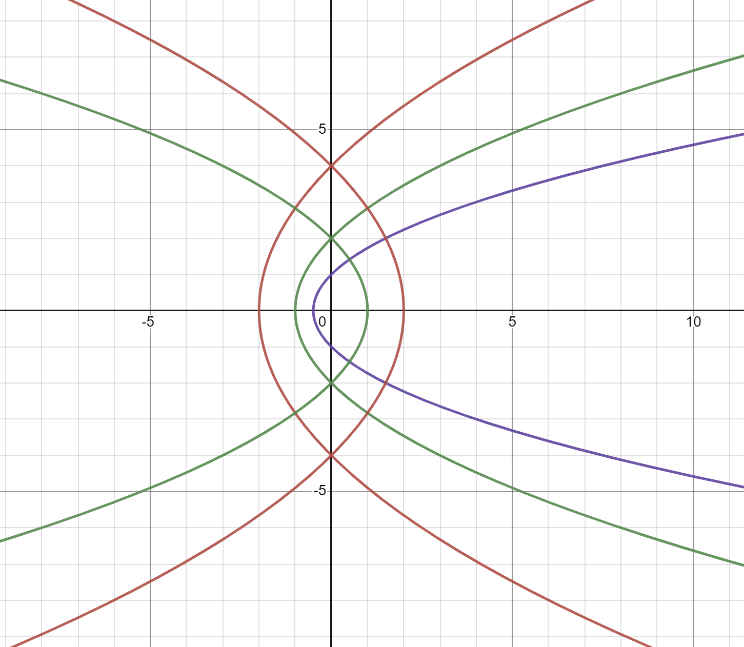
A self-orthogonal family

Show that this family of curves is orthogonal to itself: . (Hint: divide the curves into two families, one with and the other with .) Here’s a picture showing the curves for (opening rightward) and (opening leftward).

Problems due Monday 5 Feb 2024 by 1:00pm

Problem 03-01

Homogeneous; linear quotients

• (a) Solve the homogeneous equation .
• (b) Solve using linear quotients.

Problem 03-02

Reduction

The differential equation is missing both and . It can therefore be solved by reduction in ways. Solve it using both methods, and check that your solutions are equivalent to each other.

Problem 03-03

Swapping roles

Reverse the roles of independent and dependent variables and to solve:

• (a)
• (b)

Problem 03-04

Integral curves of homogeneous equation

Consider the integral curves of a homogeneous equation. Take a straight line through the origin. Show that this line crosses all the integral curves at the same angle of intersection.

Problem 03-05

First-order families

The family of curves solving a first-order linear differential equation has the general form . Now suppose we start with a family of curves in this form. Find the differential equation corresponding to this family and show that it is first-order linear.