Differential Equations - Packet 04

Functions and differential equations

Excursus: functions, derivatives, integrals

Differentiation and integration are learned as “inverse processes” in calculus, and yet this relationship tends to obscure a fundamental asymmetry between the two concepts. Differentiation has a geometrical meaning that does not rely on the concept of a function, whereas integration cannot be formulated properly without the concept of a function and naturally leads to it.

Given any equation involving and , we may consider the set of points whose coordinates satisfy the equation. For most reasonable equations, this set of points is a curve. Any point on a curve may be associated with a slope, which is the data of the direction of the curve at that point. It is equivalent to the data of the direction of the tangent line passing through the point.

(This association of point to line does not itself have to be a function, since a curve that crosses itself at some point may have two directions associated to the same point, which is disallowed for functions. Incidentally, the example of a curve crossing itself is a good illustration of a problem for the functional perspective which does not obviously have to do with infinity.)

The concept of direction line is a geometrical way of thinking about the derivative, and arguably it is more fundamental than the notion of rate of change. The direction line relates to equations and curves solving the equations. The idea of direction line is also a basic element in the idea of differential equation, since the direction of the direction line is expressed by a relationship between differentials and . One could say that a first-order differential equation is an equation involving points as well as the direction lines at those points. A solution to a differential equation is just a curve whose direction line satisfies the differential equation.

The important point here is that the idea of function is somewhat foreign to the concept of derivative and differential equation, at least when the latter are thought of geometrically.

What is a function? A function is a rule, procedure, or method taking inputs to outputs. The essential feature of the idea of function is the difference between input and output, namely the temporal priority of input along with the movement to output according to a specific pattern.

The essence of derivative (direction line) and differential equation (equation involving and ) in no way depends on a preferential treatment of as input and a patterned movement to as output.

Such is not the case for integration! The essential idea of integration depends on an inequity between the variables, between which is the independent, prior, input variable, and which is the dependent, posterior, output variable. The essential idea of integration is to sum up the values of the output with a sum that is weighted by the “quantity of inputs” for which the output has each value. The usual integration in calculus takes the total or sum of outputs weighted by the quantity of input near each input value .

A modern consequence of these conceptual differences between derivatives and integrals – between directions and summations – is that modern specialists in algebra and parts of geometry make far greater use of derivatives than they do integrals, whereas modern specialists in analysis, the discipline that studies generalizations of the concept of continuous function, are equally concerned with integrals as with derivatives.

So far our work with differential equations has mostly treated and on an equal footing. The main exception is that we have sometimes invoked the chain rule, which depends specifically on the function idea (it is about the composition of functions).

There are many reasons to adopt the functional viewpoint. Most applications of differential equations in mathematical models of physical phenomena rely on this viewpoint. Part of the reason for this is that functions are essential to the concept of rate of change, for which time is a natural independent variable, and functions are used to specify the values of physical quantities at each point in time. The “dynamical system” viewpoint is connected to this one. Numerical techniques are, furthermore, normally framed in functional terms. For these reasons the functional viewpoint is prevalent, ubiquitous, even tacitly assumed, in all applied math contexts.

Another reason to adopt the functional viewpoint is that functions give a type of structure that can encompass both algebraic and non-algebraic relationships. For example, trig functions express geometric relationships, and through the use of functions, algebraic and geometric relationships and quantities can be combined in a single equation. Furthermore, the solutions of differential equations themselves can be incorporated with algebraic and geometric functions in a single equation. For example, or Bessel functions could be included.

In short, when we are interested in mathematical quantity, over and above quality (i.e. abstract structures such as algebraic rules), and we wish to cast everything in terms of quantity, it is useful to adopt the functional viewpoint. We embrace the functional and quantitative viewpoint now and for the remainder of the course. To emphasize this transition, we now write ‘’ by default for our independent variable, and , , , , etc. are all considered to have a functional dependence on .

Initial value problems

A first-order differential equation, from the functional viewpoint, is given by a function that specifies the numerical values of the derivative in terms of the values of and . The ODE itself is . A solution to the ODE is a differentiable function that satisfies the equation.

Notice: a solution does not mean an equation or anything we might understand or know how to calculate. On the other hand, a solution is now assumed to be a function that returns numbers; this means, for example, that it cannot ever return infinity, since that is not a number.

Since the idea of a differentiable function is easy to define with perfect logical precision, we can ask about a differential equation the logical question of how many solutions exists. If there are infinitely many, we can ask whether there are conditions we can specify that guarantee existence of a unique solution. Taking the functional viewpoint, we typically would like to express such conditions in terms of inputs and outputs of the solution function.

An initial value problem (IVP) is a problem where we specify an initial time and initial values of the function and possibly a number of its higher derivatives: , , , and ask whether there exists exactly one differentiable function solving the differential equation and that has these initial values.

The idea of initial value problem also applies in numerical analysis, which is concerned with the development of algorithms that generate approximate solutions for use by computers, because these algorithms typically build approximate solutions by iterating a procedure which extends a partial solution into future time intervals.

Functional viewpoint and IVPs: pathological phenomena

The class of differentiable functions may be easy to define with logical precision, but some innocuous-looking differential equations, even some with reasonable “families of integral curves,” exhibit pathological behaviors from the functional viewpoint.

Vertical asymptote means blowing up: non-existence It is easy to find a differential equation with IVP starting at whose functional solutions go to infinity in finite time. When this happens, the solution is said to blow up.

Example

Solution that blows up

Consider the IVP:

This is a separable differential equation. Assuming , we can solve it: . From the algebraic viewpoint we had been using, the solution to the ODE is the family of curves , and there is no particular problem with this family.

Now write the solution as a functional solution and solve for the constant using the initial condition :

Look what happens as time evolves: for , the function is well-behaved. But as we have . In other words, blows up at . There is a solution to the IVP (and in fact it is unique when it exists), but the solution cannot be extended beyond the range .

This blow-up behavior is not weird algebraically, but functionally it is undesirable, since the solution function does not exist beyond a certain time .

Notice that if the ODE is replaced by , then the solution is , which does not blow up for . (Although it does blow up for .)

Artificial functional solutions: non-uniqueness Another kind of problem can arise in the functional perspective with a differential equation that poses no difficulties from the algebraic perspective. The problem is that mere “differentiability” is not strong enough to separate out functions that are the same in first derivative, but their higher derivatives may fail to exist.

Example

Once-differentiable functions given piecewise, non-uniqueness

Consider the IVP:

This is a separable differential equation: so . Solving this explicitly: , and is a solution satisfying .

But look! Here is a piecewise function, for each , that also solves this IVP:

Clearly this is a solution for . Considering , we have:

and therefore does exist, namely , and the ODE is satisfied everywhere.

Notice that does not exist at !

Furthermore, the piecewise solutions are not given by a single equation with parameter, so they do not qualify as a “family of curves” according to our previous usage in the algebraic viewpoint.

The family of functional solutions is wild! It can start to increase parabolically at any random time of our choosing. Clearly there is no unique solution to this IVP in the class of differentiable functions. Notice that this non-uniqueness is a local problem, meaning that there is no interval around for which there exists a unique solution. If we desire local uniqueness, then either the differential equation itself is not acceptable, or else our class of functional solutions is too big.

By adopting the functional perspective, we restrict ourselves to objects that are better behaved in one sense – they are well-defined and avoid infinity – but they are worse behaved in another sense: they may exhibit strange behaviors that no algebraic families of curves would, such as non-differentiability, piecewise definitions, random bifurcations, and so on.

Consider the fact that does not exist. Can we fix our problem by restricting functional solutions to the class of functions that are infinitely differentiable, meaning that all their higher derivatives exist and are continuous?

No!!

Example

Infinitely differentiable: not enough for uniqueness

Consider the IVP:

This differential equation is separable, and the solution family is calculated to be for . We can also check that is a solution too.

But look! Here is a piecewise function, for each , that solves the IVP:

At we have for any . For example, from the right , and this limits to zero as . (It is not trivial to prove this, but intuitively the exponential goes to zero much faster than does.)

All these functions are infinitely differentiable, they all satisfy the IVP, and yet they differ from each other for any (for differing values).

Exercise 04A-01

Hopping from a line

Consider the IVP: . Show that the (differentiable) functional solutions can extend along the line for arbitrary time in the forward direction, and at some moment deviate from the line following a certain parabola. Can the same happen in the reverse direction?

You are encouraged to understand the differential equation using the Desmos graph at https://www.desmos.com/calculator/sdxp7or83y.

Picard-Lindelöf Theorem: local well-posedness

Our only major theorem in this course is due to Cauchy, Lipschitz, Picard, and Lindelöf. Usually Picard is given most of the credit, but frequently it is called the Picard-Lindelöf theorem.

Picard-Lindelöf Theorem

Suppose the IVP is given by the function and initial value :

and suppose that has the following properties: there is some rectangle containing , and numbers such that:

Then there exists a unique local solution to this IVP.

Here the precise meaning of local solution is that there is some interval for which a solution exists. The local solution is unique in the sense that any other local solution must agree with this solution on some interval (possibly smaller).

Variants of Picard-Lindelöf

• If we know that and are both continuous on some rectangle containing , then there exists a unique local solution to this IVP.
• If we know that and are both bounded on some rectangle containing , then there exists a unique local solution to this IVP.

These statements follow from the first version using the Mean Value Theorem and some topological arguments that we omit.

Picard-Lindelöf does not prevent blowups!

The Picard-Lindelöf theorem only provides local solutions, meaning some interval which is potentially microscopic on which the solution exists. These intervals could become arbitrarily small as you approach a blowup point. They do not guarantee solutions that extend beyond a blowup point!

On the other hand, the Picard-Lindelöf theorem does prevent the artificial piecewise solutions we have seen which exhibit non-uniqueness. How? Those IVPs do not meet the conditions of Picard-Lindelöf! In other words, instead of trimming away bad functional solutions, the theorem excludes those IVPs because the differential equations themselves are excluded.

Example

Picard-Lindelöf frequently not applicable

The IVP does not satisfy Picard-Lindelöf. We have , and this is neither continuous nor bounded on any interval containing . So the “Variants” of Picard-Lindelöf do not apply. Furthermore, the difference quotient can be made arbitrarily large by letting it approximate this partial near , so the original Picard-Lindelöf does not apply either.

Conclusion: the Picard-Lindelöf theorem restricts us to IVPs with such that is nicely behaved near the initial data . Critically, this means the partial should be nicely behaved there too.

Picard iteration

The Picard-Lindelöf theorem is proven by developing a sequence of functional solution candidates, and showing that they converge to a real solution, and furthermore that any other solution must converge (locally) to the same one. Functions in this sequence are called Picard iterates because the sequence is produced by an iterative process.

The Picard iteration procedure can be computed by hand for some interesting cases, and it is worthwhile to do so. To that end, let us set up the process in general.

From the functional viewpoint, an IVP is given by and . It is convenient to assume that . (If this is not the case, you can change variables and write a new IVP in the new variables that does satisfy this property.) So the IVP is now and .

Suppose is a solution to the IVP. Integrate both sides:

Now suppose is a function that satisfies the above integral equation, and differentiate both sides. By the Fundamental Theorem of Calculus, we obtain and . Therefore, the integral equation above is equivalent to the original IVP.

Notice that this translation to an integral equation relies critically on the functional viewpoint!

Ponder the format of this integral equation. It says that if we apply the operation to the function , then we get back the same function . In other words, is preserved or fixed by this operation.

The general strategy to show that there is a unique solution is to show that there can be only one fixed point of this operation acting upon the class of differentiable functions. (The reason is that the operation is “shrinking,” in a sense that we cannot explain fully here, but the rough idea is that it pulls candidate functions closer and closer together.)

The strategy to show that a solution exists is to start with any candidate function and apply the operation repeatedly, and the candidate will be pulled closer and closer to the fixed point of the operation, namely to the solution of the IVP. To notate this, let be any initial candidate solution. Then we define:

We expect that as , for a solution to the IVP.

Example

Picard iteration can yield an exact solution

Consider the IVP . Change variables to and get the IVP and . Set and iterate:

So we conclude that is given by the power series

and the coefficients are defined recursively by , . This recursion relation is solved by the general term , so we have:

We found an exact solution by:

• computing Picard iterates,
• observing a growing power series,
• identifying a recursion relation,
• solving the recursion relation for the general coefficient,
• recognizing a known power series.

Sometimes the last step or two cannot be accomplished, but in principle the first three steps can always be done.

Problems due Monday 12 Feb 2024 by 1:00pm

Here is a Desmos page that graphs slope fields: https://www.desmos.com/calculator/p7vd3cdmei The problems below contain some more specific links.

Problem 04-01

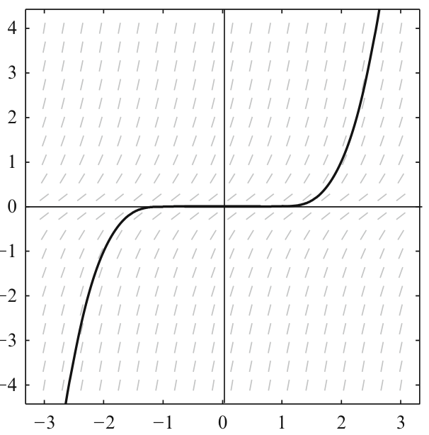
Hopping from the -axis

Consider the IVP: . Analyze the functional solutions to this IVP. Extend your analysis to as well. This Desmos and picture might help you: https://www.desmos.com/calculator/n8yfpnshxd

Problem 04-02

When does Picard-Lindelöf apply?

Which of the following IVPs satisfy the conditions of the Picard-Lindelöf theorem?

• (a)
• (b)
• (c)
• (d)

Problem 04-03

Understanding existence and uniqueness

Consider the IVP of the previous problem, part (c):

• (a) Precisely which initial data are such that the Picard-Lindelöf theorem is satisfied, guaranteeing existence and uniqueness of local solutions? Which would ensure failure? (Your answer would also answer Problem 04-02(c) as a specific case.)

• (b) Solve the homogeneous differential equation very carefully (double check your solution set). Exactly which solutions blow up? (For this question, specify the solutions using initial conditions living either on the -axis or on the -axis.)

For both parts of this problem, you should graph the slope field using Desmos: https://www.desmos.com/calculator/gypelekic6. For part (b), you should graph your solutions on top of the slope field. It is recommended to implement your constant as a slider so you can move the solution curves around. (No need to submit your graphs.)

Problem 04-04

Picard iterates

• (a) Compute the Picard iterates up to , starting with , for the IVP:

• (b) Compute the Picard iterates up to , starting with , for the IVP: