Differential Equations - Packet 06

Numerical techniques

This packet is about methods that can be used by a computer to produce numerical solutions to first-order IVPs, and more specifically, methods that are usually guaranteed at least some success and rely only on the ability to calculate the derivative by evaluating a given function . These methods work by starting at the initial value and iteratively building a solution, stepping forward in time to propose candidate values that depend on evaluations of at various points as well as the values at previous times.

Extending partial functions in time vs. refining complete functions to higher orders

In Packet 10(?) we will consider approximation methods of a different nature, namely power series (for example as produced by Picard iteration), and Fourier series.

Instead of building a solution out across time, producing future solution values during the process, these methods produce coefficients for infinite series that converge to the solution. A systematic approach along these lines was developed by Parker-Sochacki.

The methods of this packet produce partial functions defined only up to a given time, and these partial functions are not updated in the past (at least not much), rather they are extended ever further forward. The methods of Packet 10 produce complete functions, namely as partial sums of the series, but the values at early times are subject to revision as later terms are added, meaning that the complete functions are changed across all time with each further iteration.

Euler’s method

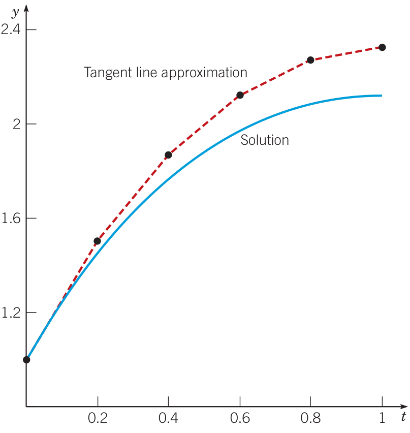
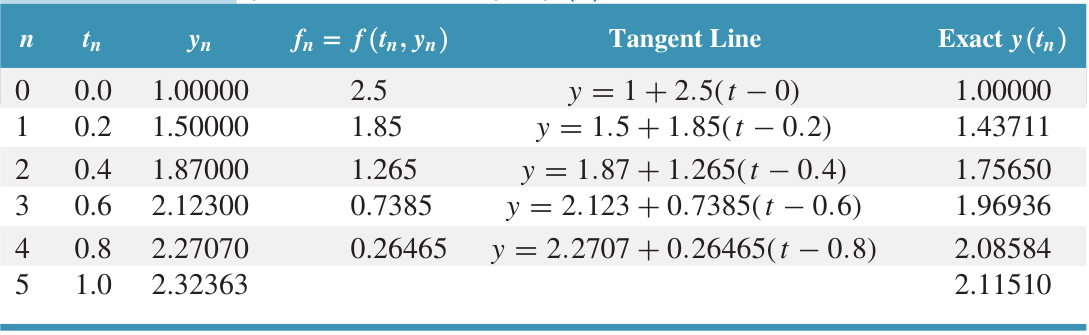
The simplest imaginable algorithm for solving an IVP numerically is attributed to Euler. The method is simply to follow tangent lines.

Suppose the IVP is given by

We construct an approximate solution iteratively, using a step size of , as follows:

The process is iterated until reaches the desired stopping time .

Question 06-01

Euler’s method practice

Consider the IVP:

Use Euler’s method to compute an approximate solution up to with step size . Show all four steps of the partial solution.

Euler’s method is not always accurate

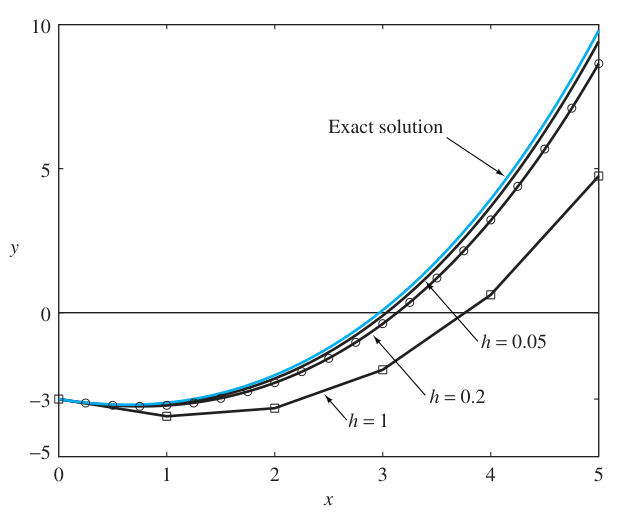
The Euler method is very easy to implement on a computer or even a programmable calculator. It is frequently very inaccurate, however, since the errors can build up rapidly. With exponentially growing solutions, for example, the Euler method will fall far behind in a short time, even with a small step size.

Exercise 06A-01

Euler’s method struggles with large slopes

Consider the IVP:

Desmos: https://www.desmos.com/calculator/gbijdaprd3

• Use Euler’s method to compute an approximate solution at the times using .
• Use Euler’s method to compute an approximate solution at the times using .
• By considering the slope field, possibly in conjunction with an exact solution, can you explain why the approximate solutions differ so much at ?

Exercise 06A-02

Euler’s method becomes the left-endpoint rule

Show that if the ODE is amenable to solution by direct integration, meaning actually does not depend on , then Euler’s method amounts to the left-endpoint rule for integration of .

Heun’s method

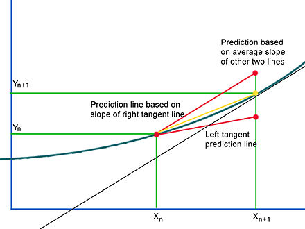
The function allows us to access slope values anywhere, but in Euler’s method we only use the slope value at the starting point of each step.

Instead of taking the slope at to extrapolate from , we can take the slope at both and . Well, this can’t quite be done because we don’t know in advance, but we could use the Euler method to forecast initially and call this , then take the slope , and finally compute the average slope at the two points. Then we extrapolate our next step from using this average slope instead of the slope . We obtain the formula:

This formula can be iterated from with step size until reaching the desired stopping time .

Question 06-02

Heun’s method practice

Consider the IVP:

Use Heun’s method to compute an approximate solution up to with step size . Show all four steps of the partial solution.

Question 06-03

Comparing methods

Solve algebraically the IVP as in the previous Questions: . Make a table of values to compare the results of Euler’s method, Heun’s method, and the exact solution. Write the percent error next to the values from the approximation methods. Create a final column that includes the percent difference between the approximate solutions. Can this column predict the percent error without knowing the exact solution?

Heun’s method becomes the trapezoid rule

If the ODE is amenable to direct integration, so actually does not depend on , then Heun’s method amounts to the trapezoid rule for integration of .

Runge-Kutta methods

The basic idea of Heun’s method is to capture more information from ahead of the given step . We want to use these candidate slope values in the vicinity of the point to better approximate the exact average slope, namely the value that gives the slope of the secant from the current step to the exact solution at the next step.

The idea of Heun’s generalization of Euler’s method can be extended to any number of stages, where a stage refers to the number of ‘forecasting’ evaluations of the function that are required for each step. The Euler method is 1-stage, and the Heun method is 2-stage.

The general name for -stage methods that generalize Heun’s method is Runge-Kutta methods. The most famous and widely used Runge-Kutta method is a choice of 4-stage method that sometimes is simply called the Runge-Kutta method. (So if no stage number is specified, this 4-stage method is implied.)

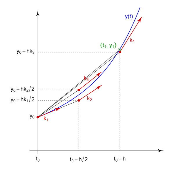
For this method, we sample 4 slope values, called :

• – slope at current step
• – slope at the Euler forecast using , half step
• – slope at the Euler forecast using , half step
• – slope at the Euler forecast using , full step The final value for the next step is then:

In other words, the slope we use to compute the next step is a weighted average of various slopes in the ‘future vicinity’ of .

The possibilities are endless

There is no simple explanation for the choice of sampling locations and the choice of weights used for the final slope. Other possibilities are also studied.

Exercise 06B-01

The Runge-Kutta method becomes the Simpson rule

Show that if the ODE is amenable to direct integration, so actually does not depend on , then the Runge Kutta method amounts to the Simpson rule for integrating .

Recall that the Simpson rule comes from fitting parabolas. It is given by:

Adams method: multistep: polynomial fitting

The methods studied so far, Euler, Heun, and Runge-Kutta more generally, have been single step methods. This terminology means that each step of the iterative process makes use of the data of a single previous step. In the formulas above, was determined (through some process) by the value of alone.

A multistep method uses the data of multiple previous steps to estimate the next step. For example, a 3-step method would use , , in order to estimate .

Runge-Kutta is not multistep

Do not confuse the use of multiple estimated slopes with the use of multiple previous steps!

To simplify the formulas for multistep methods we define , so is a scalar quantity representing the slope given by the ODE at the previous step .

The most natural and common multistep method is produced by fitting a polynomial of degree to the slopes at the previous steps, namely to

and then extrapolating forward on this polynomial. This is called the Adams method.

Example

Two-step Adams method

We seek a parabola with three properties:

The graph of this parabola will pass through the previous step and match the slope of the ODE at the two previous steps and .

To find the coefficients of , first solve the system:

(Observe that the second and third equations are independent of the first, so they should be solved initially and the result used to compute from the first equation.) Obtain:

Then the next step value is given by evaluating the polynomial at :

This is the Adams formula for in terms of and .

Exercise 06B-02 = Problem 06-02

Three-step Adams method

Compute the formula for the three-step Adams method.

Errors

Next we consider the accuracy of the above methods in a quantitative way. It is important to learn some vocabulary to refer to various sources of error, especially as users of numerical ODE solver packages.

• Local truncation error is error arising in the single step of the iterative solution procedure, assuming that the starting values of the previous step are accurate (or taking them for granted as initial conditions).
• Global truncation error is the accumulation of local truncation error as the procedure is iterated over steps.
• Round-off error is the accumulation of error due to finite-precision arithmetic operations performed along the way, as the procedure is iterated over steps.
• Total accumulated error is the difference between the approximate and the exact solutions at the ending time. It is satisfies where is the step number of the ending time.

The global truncation error is (in principle) some function of the local truncation error, since it measures the accumulation of that error.

Truncation errors are due to the mathematics of the approximation procedure. For a coherent procedure, the truncation errors should vanish in the limit as and the approximation converges to an exact solution. Truncation error is therefore reported in terms of powers of .

The “Big-O” notation is used to describe how quickly as . The ‘’ can be read as “order.” We say , read “ has the order of ,” when for some and .

With the Euler method, for example, we will see that and , so the Euler method is called a first-order method. It turns out that the Runge-Kutta method has , and it is therefore called a fourth-order method. Any method with is at worst a -order method. The goal in constructing Runge-Kutta methods is to minimize the number of calls to the function while maximizing the order of the global truncation error.

Local truncation error for the Euler method

Assume that are all continuous in the region of interest. Suppose is an exact solution to the IVP. Then , and the chain rule gives us:

Now consider the Taylor series with remainder of expanded around :

where is some value giving the remainder term.

The local error for Euler’s method is therefore:

So our local error bound is proportional to and to . Letting be the maximum of in the region of interest, we see that .

Local to global is not trivial

The relationship between local and global truncation errors is not quite as simple as it appears. You cannot derive that global is always one order lower than local by multiplying the global error by the number of steps (i.e. by ). The problem is that the constant appearing in the local truncation error order equation can vary dramatically over the course of a solution – it depends on the slope field in the region. To derive the global error from the local error, you have to know how quickly the local error can vary.

Adaptive methods

Some regions of the slope field demand a smaller for sufficient accuracy (for a sufficiently small local truncation error) than other regions. If the smallest necessary is chosen, the calculations will be much slower than would be possible in regions where an this small is not needed. Therefore, using a fixed step size is usually not the best practice for real implementations of numerical ODE techniques. Rather, it is best if the implementation can estimate the accuracy of its own calculation, and use this estimate to adjust the step size for an optimal balance of accuracy and efficiency.

A standard method to adapt the step size dynamically is to use a solution procedure that is one order better than required, together with a solution procedure that is just as required, and to compare the outputs. The difference of outputs gives an estimate of the actual local truncation error. It is a sort of detector of that error. When the local truncation error estimate gets too big, the step size is reduced; when it’s smaller than necessary, the step size is increased and the computation speeds up.

A very popular numerical solver called “RKF” (for Runge-Kutta-Fehlberg) uses a Runge-Kutta fourth-fifth order coupled procedure, where the data of the fourth-order procedure is reused for the fifth-order procedure and just a little more data added by function calls to . A famous FORTRAN implementation of this is called RKF45.

In Question 06-03 you already considered a part of this process. The Heun method uses the data from the Euler method, calling the function one more time. Since the Heun method is more accurate than the Euler method, the Heun solution can be used as a substitute for the exact solution, and the difference between Heun and Euler outputs gives an estimate for the local truncation error of the Euler method. If in this problem you had adjusted on the fly, depending on the error estimate, you would have had an adaptive method.

Stability and stiff problems

Another concept is worth pondering in preparation for a scenario where you have to implement an ODE solver package.

• An IVP is stable if errors in the solution tend to decrease over time.
• An IVP is unstable if errors in the solution tend to increase over time.

Errors generated at early times in the solution approximation will propagate through the solution to later times. For some situations, the errors are shrinking down as the solutions are converging together. For other situations, the errors are growing, perhaps rapidly and without bound, as solutions are diverging from each other.

A perhaps unexpected fact is that an IVP can be stable in itself, and yet a solution procedure can generate instability. This is where exact solutions to the IVP that start with some difference end up converging together, but approximate solutions using the procedure actually end up diverging.

This means that the step size may have to be controlled to prevent the introduction of instability. A problem is called stiff when the step size needed to maintain stability is smaller than the step size needed to maintain numerical accuracy (local truncation error). Frequently a backward differentiation method is the best approach for a stiff problem; see Problem 06-03 to learn about those.

Problems due Monday 26 Feb 2024 by 1:00pm

Problem 06-01

Runge-Kutta practice

Find an approximate solution to with using the standard fourth-order Runge-Kutta method described above, up to , with a step size .

Problem 06-02

Three-step Adams method

Compute the formula for the three-step Adams method.

Problem 06-03

Euler method accuracy: small enough step size

For the IVP of Question 06-01, find (with justification!) a value of that is small enough to ensure that the Euler method gives a solution at which is accurate to within of the exact value.

Problem 06-04

Backward Euler method

There is a family of procedures called “backward differentiation methods.” The backward Euler method specifies implicitly by the following equation:

It is called backward because the slope used here is the slope of the future step . There are backward versions for all the Adams methods. (The forward Adams methods are also called Adams-Bashforth methods, while the backward versions are called Adams-Moulton methods.)

For this problem, use the backward Euler method to approximate the solution to the IVP up to , with . (See Boyce et al. text for examples if desired.)