Differential Equations - Packet 09

Inhomogeneous theory

The solution method for homogeneous second-order linear equations is part of the solution method for inhomogeneous ones. The homogeneous theory provides the parameters, while a single “particular” solution to the inhomogeneous equation provides an “offset.” This offset shifts the vector space of solutions to the homogeneous equation over to the affine space of solutions to the inhomogeneous equation.

The situation is exactly akin to that of solutions to homogeneous and inhomogeneous matrix equations, and . The solutions to form a vector space, namely the null space of . The solutions to form an affine space that is given by adding a single particular solution satisfying to the null space of . The reason: any two solutions to differ by a solution to . Therefore the affine space of all solutions to can be obtained by shifting the vector space of solutions to over by an offset which is one particular solution .

A generic second-order linear inhomogeneous ODE is given as follows:

This ODE determines a corresponding homogeneous ODE:

Given two “independent” solutions and to the homogeneous ODE, any linear combination of them is also a solution, and a complete family of solutions is determined as their span:

Given a single particular solution to the original inhomogeneous equation, the complete family of solutions to the inhomogeneous equation is the span for the corresponding homogeneous equation shifted by that particular solution as an offset:

Variation of parameters

The method of variation of parameters is to change a constant value parameter like into a variable function , and see whether we can cook up an appropriate so that the solution is still a solution with this variable parameter .

Discovering a second solution

Suppose we are given a single solution to the homogeneous equation . We know that is also a solution, but it isn’t independent of . We would like to find another, independent, solution which will span (along with ) the complete set of solutions.

Let us propose the hypothesis that there is a solution for some function of .

This solution will be independent of provided is not constant. The trick is to supply some additional constraints on that make it feasible to solve for what must be, given that solves the equation. These constraints emerge from the process of plugging into the equation and expanding the product and chain rules.

which we continue to solve as by separation of variables:

(We have allowed an abuse of notation by letting indicate any particular antiderivative, understood to be a function of .) By running these equations backwards, we find that if , then is indeed a second solution.

This method always works! That is, it provides a second solution in terms of a first solution and two integrations.

This method is enough to explain the factor appearing in our secondary solutions to linear equations with constant coefficients and repeated roots:

Example

Variation of parameters: double repeated roots

Suppose is an ODE with and therefore and is a repeated root. We have seen that is one solution. Let us change the parameter in the family to a function and plug it in:

This quantity is zero when , which happens when and . It is enough to consider the specific case because the other parameters are already accounted for when we take the span to obtain the complete set of solutions:

Example

Variation of parameters: second nontrivial solution from trivial guess

Problem: Find a complete family of solutions to the ODE given by .

Solution: This ODE is reducible to first order because does not appear. However, let us use variation of parameters to solve it. Write it as . Notice first that is a (rather trivial) solution. Look for a second solution of the form . Using the formula, we have:

So is a second solution, and the complete family is given by .

Question 09-01

Variation of parameters: triple repeated root

Suppose , and suppose for some . Use variation of parameters to find two (independent) additional solutions besides .

Question 09-02

Variation of parameters: Legendre second solution

The Legendre equation for is . One solution is . Find a second solution.

Exercise 09A-01

Variation of parameters: double repeated root, inhomogeneous

Find a complete set of solutions to the ODE given by .

Exercise 09A-02 = Problem 09-02

Variation of parameters: second solution from one obvious.

Find a complete set of solutions to the ODE given by .

Particular solution of inhomogeneous

The same strategy, with a complication, will provide a particular solution to an inhomogeneous equation by variation of the parameters of the complete set of solutions to its corresponding homogeneous equation.

Suppose is the complete family of solutions to . We seek a particular solution to . Let us propose the hypothesis that a particular solution has the form

As before, we substitute this form for into the equation and eliminate the consequences of and being solutions. We compute:

Now for the new complication of this method. It will be very convenient to add the additional constraint that . This is a constraint on the possibilities we are hypothetically contemplating for , meaning for and . We are not required to add this constraint, but we will discover that it is not too strong in the sense that we can always succeed in finding a solution with this constraint, and it greatly simplifies the algebra, so we do so. The first terms in brackets in the expressions for and therefore disappear.

Plugging the rest back into the equation, we find:

So it will be enough to solve this last equation simultaneously with our constraint equation, namely to solve the system:

Given , this is a simple system of linear equations in two unknowns and we can solve for them explicitly:

Therefore, setting

we have a solution .

Example

Solving an inhomogeneous equation

Problem: Find a complete set of solutions to the ODE given by .

Solution: The corresponding homogeneous ODE is , which has characteristic equation , and its general solution is therefore .

To find a particular solution to the inhomogeneous, we consider varying parameters. Let and . Using the formulas above for and , we compute:

(Notice, again, that we will not need the integration constants, since those will lead to repeat part of the homogeneous solution.)

Adding the particular inhomogeneous solution to the general homogeneous solution, we find the complete family:

Exercise 09A-03

Solving inhomogeneous linear ODE

Find a complete set of solutions to the ODE given by .

Exercise 09A-04

Solving inhomogeneous linear ODE

Find a complete set of solutions to the ODE given by .

Exercise 09A-05

Solving inhomogeneous linear ODE

Find a complete set of solutions to the ODE given by , where are constants.

Exercise 09A-06

Superposition and sums of forcing terms

Find a complete set of solutions to the ODE given by .

(Hint: add two particular solutions together, each solving an inhomogeneous equation corresponding to a single one of the forcing terms.)

Applications

Second-order ODEs frequently arise in physics because the laws of physics are frequently given using principles of force or energy, and these quantities are related to basic state variables (position) using second derivatives. Consider Newton’s Law:

and the Lagrange equation (having to do with energy and “action”):

Many important second-order ODEs in physics are also linear. The basic case of constant coefficient second-order linear equations gives what is called the harmonic oscillator. Harmonic oscillators arise in various branches of physics, from mechanical vibrations to electrical resonance circuits. “The” harmonic oscillator is a class of mathematical models (with assorted parameters and forcing functions) that describe the various real oscillators in physics.

Damped harmonic oscillator

• A mechanical simple harmonic oscillator can be formed with a mass sliding frictionlessly over a surface, attached to a spring anchored to a wall.
• A basic damped harmonic oscillator can be formed by adding a “dashpot” that provides resistance to motion. Ordinary friction provides a resistance force that is independent of velocity, whereas a dashpot provides resistance that is proportional to velocity.

Let describe the position of the mass over time, with when the mass is resting statically. The spring force is given by , and the dashpot force is , where gives the spring constant and gives the dashpot constant. By Newton’s Law, , so we have . In other words:

Undamped case The case corresponds to the absence of any dashpot. The resulting equation has characteristic equation with solutions . The complete set of solutions is therefore:

For application purposes, it is useful to consider formulas like the above in a different format, using a trig identity:

Considering the form , the parameter is called the amplitude, is the angular frequency or circular frequency, and is the phase angle or phase lag. The angular frequency is related to the true frequency and the period by:

The relation can be summarized by saying that the sum of sinusoidal functions with the same frequency is also a sinusoidal function.

You are encouraged to manipulate the parameters of on Desmos: https://www.desmos.com/calculator/i9tpybmra9

Adding damping Now suppose we allow . Let us write and , so then the ODE takes the form:

Let use write . The solutions to the characteristic polynomial are and when , and and when .

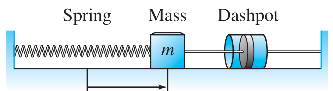
Case 1: Overdamping When , there are two real roots. The solutions are negative exponentials and quickly die out:

https://www.desmos.com/calculator/yn9bcqflf9

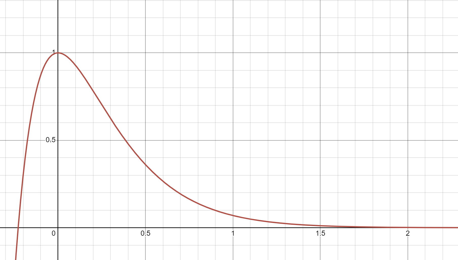
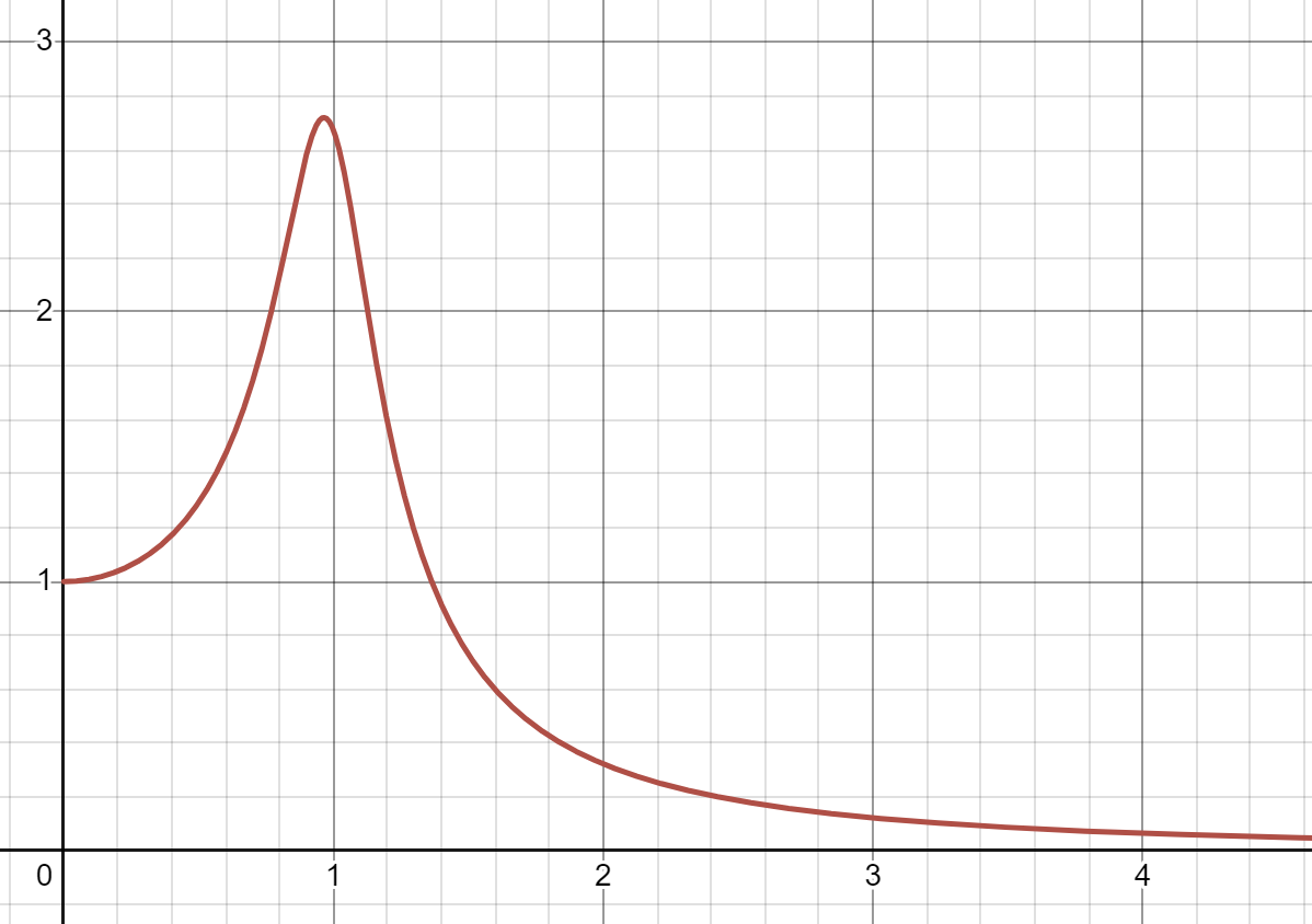
Case 2: Underdamping When , there are two imaginary roots. The solutions are decaying sinusoidal with continued oscillations that decay in amplitude:

where we set . https://www.desmos.com/calculator/s9oyz7gtot

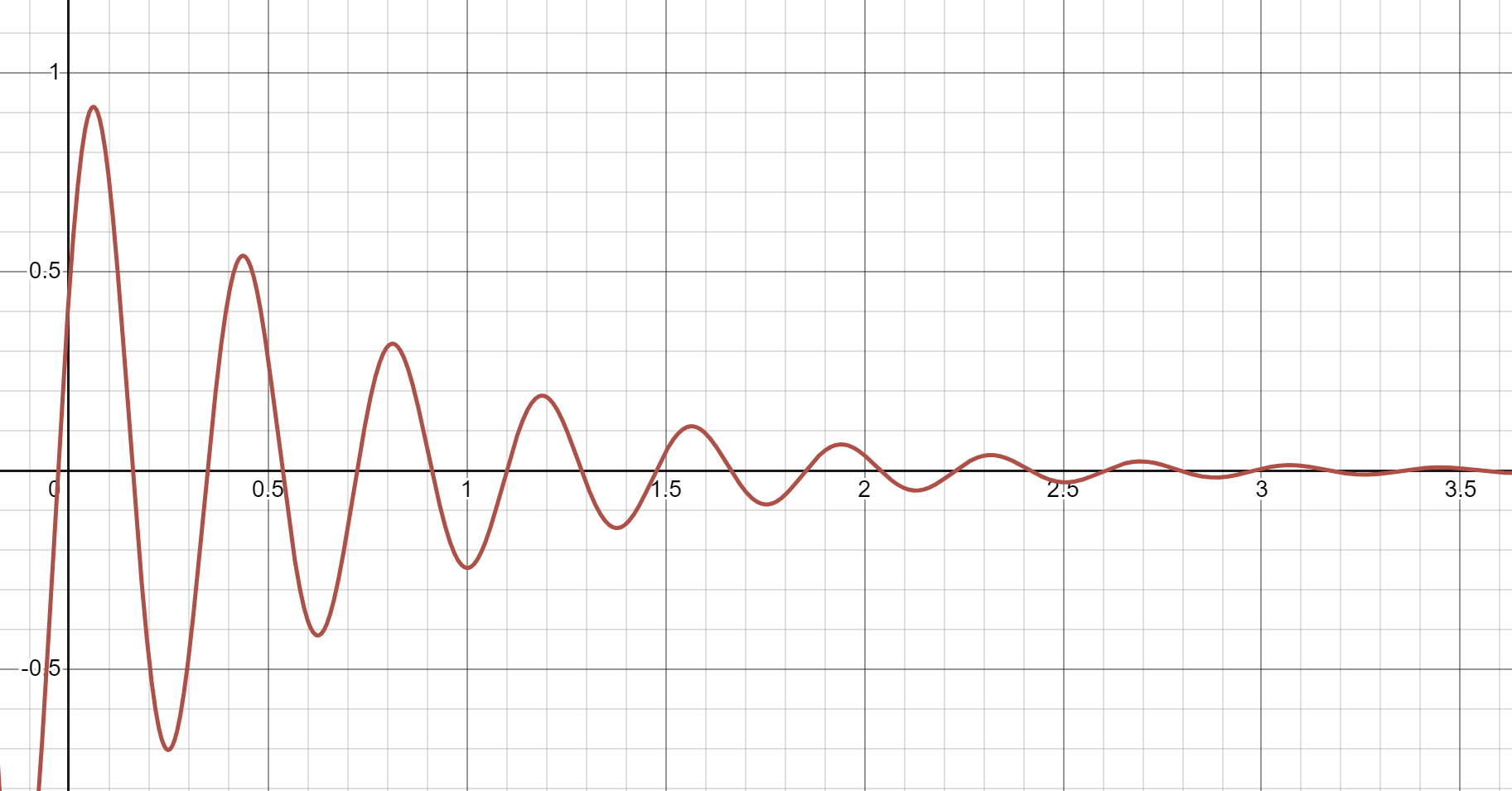
Case 3: Critical Damping When , the situation is that of repeated roots, . The complete family of solutions is therefore:

Rewriting in terms of initial , starting at rest:

https://www.desmos.com/calculator/mjjyd54yf3

This critical damping case is very important in practical applications. The effect of critical damping is to dampen out oscillations (1) as quickly as possible, (2) without allowing “overshoot.”

Driven harmonic oscillator

In this section we consider more closely the effect of a sinusoidal forcing function, at first without any damping. Our ODE becomes:

We know that this ODE has a complete family of homogeneous solutions given by

Here we are writing for the angular frequency of the forcing function, while we write for the natural response frequency of the system.

Exercise 09B-01

Driven undamped harmonic oscillator amplitude

Show that the above ODE has a bona fide (particular) solution given by , where

Notice! This amplitude is not free to vary as in the homogeneous case. It is determined by the driving function.

Notice something else! This amplitude goes to infinity when . The natural system response amplitude is called the resonant frequency and this phenomenon of a large response to a driving force that is oscillating in tune with the natural system frequency is called resonance. In real life, there is always some damping effect, and this will mitigate the actual infinity in the equation.

The complete family of solutions is given as usual by adding the homogeneous solutions to our bona fide solution:

Of course, the homogeneous solutions are simply superposed over the bona fide solution. (Added to it.)

The format of this solution is inconvenient because the homogeneous amplitude and phase lag is not necessarily apparent in the actual solution values , while on the other hand the initial conditions are also not apparent anywhere in the formula.

The concepts of Zero State Response (ZSR) and Zero Input Response (ZIR) are ideas from engineering that allow us to view the space of solutions in a more revealing format.

• Zero State Response refers to a bona fide solution with zero initial conditions: . We will write for this solution, where indicates the symbol for the forcing function.
• Zero Input Response refers to a homogeneous solution with given initial conditions: , . We will write for this solution, where indicates homogeneity.

In our case above, the ZSR is

and the ZIR is

The solution to any IVP will be the sum of the ZSR and a certain ZIR:

The former derives from the forcing function, and the latter derives from the initial conditions.

The purpose of these concepts is to treat the initial conditions as stimulating a homogeneous system response to the starting conditions, while the forcing function drives a particular solution (presumed starting from rest) that is layered on top. Any solution can be obtained in this way.

Exercise 09B-02

Checking ZSR and ZIR

Verify that and are given correctly.

Driven, damped harmonic oscillator

In the final case we add damping to the driven harmonic oscillator, obtaining the ODE:

The complete family of homogeneous solutions depends (as above) on cases, giving overdamped, underdamped, and critically damped solution types:

As before, here we are using , , and . These solutions are essentially in ZIR form already.

The ZSR is new and interesting. We have:

This formula shows that the amplitude of the ZSR has a distinctive peak of at the resonant frequency . At this frequency, the phase lag is . Notice that the extra term in the radical prevents blowing up at . https://www.desmos.com/calculator/hqlrgor3eb

Series RLC circuit

The current flowing around the electrical circuit with diagram: 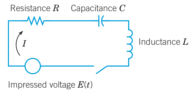is described by a differential equation that may be compared to the equation for mechanical vibrations of a mass + spring + dashpot system:

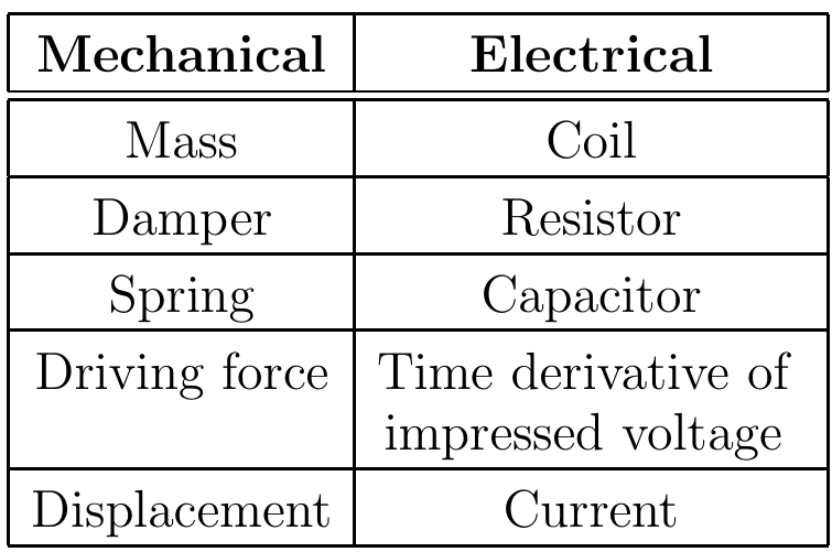
Here is a correspondence dictionary: All the theory developed above applies to such a circuit.

MIT Mathlet links

Spring and dashpot, spring is driven | Spring and dashpot, dashpot is driven | [Spring and dashpot, both are driven](https://mathlets.org/mathlets/amplitude-and-phase-2nd-order-iii/ | Spring and dashpot, mass is driven | Damped vibrations | Forced, damped vibrations | Series RLC circuit

Problems due Monday 18 Mar 2024 by 1:00pm

Problem 09-01

Superposition and sums of forcing terms

Find a complete set of solutions to the ODE given by .

Problem 09-02

Discovering a second solution

Find a formula (maybe involving integrals) for the complete family of solutions to the following ODE:

Your answer should be written in terms of the unknown function . Hint: first guess an easy solution.

Problem 09-03

Variation of parameters

Using variation of parameters, find particular solutions to the following ODEs:

• (a)
• (b)

Problem 09-04

Fourier solution

Using variation of parameters, show that the solution to the IVP

is given by .

Problem 09-05

Quasi-frequency

An underdamped harmonic oscillator vibrates at some “quasi-frequency” . This is not a true frequency because the motion is not truly periodic, due to its decay over time. Find a formula for the ratio where is the natural frequency of the undamped harmonic oscillator with the same mass and spring. Does the damped oscillator vibrate with a faster or slower frequency than the same oscillator without damping? What happens to as and thus ?

Problem 09-06

Bobbing buoy

A cylindrical buoy in diameter bobs in water with its axis vertical. The density of water is . The period of its bobbing oscillation motion is . How heavy is the buoy?