Differential Equations - Packet 14

Fourier series

Fourier series basics

A Fourier series looks like this:

The constants and are called Fourier coefficients. The summand terms and are called Fourier components or frequency components. They represent sinusoidal contributions with frequency .

A Fourier series can be viewed as having two parts, the even part and the odd part:

Even and odd functions

An “even” function satisfies , while an “odd” function satisfies .

• So is even, while is odd
• Sum rule: while
• Product rule: and while

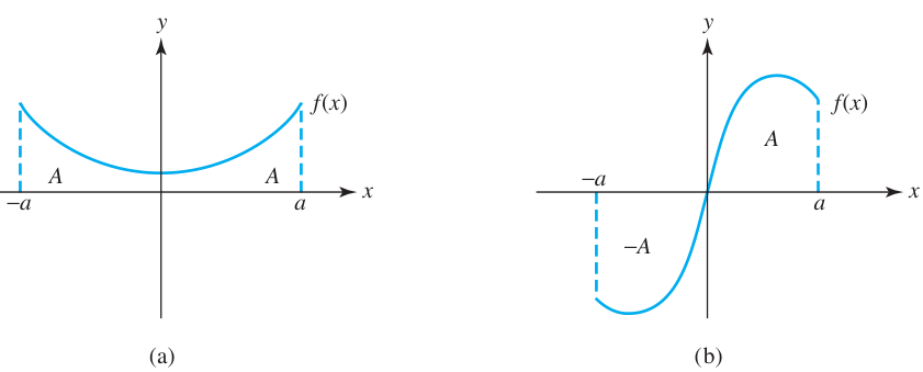
Given any function , we can write it as a sum of even and odd parts. Let , and . Then is even, while is odd, and .

Even and odd parts are uniquely determined

If then is both even and odd. But if and then and necessarily .

Question 14-01

Even and odd parts of a Fourier series

Let .

Prove that the even part is the cosine series, while the odd part is the sine series.

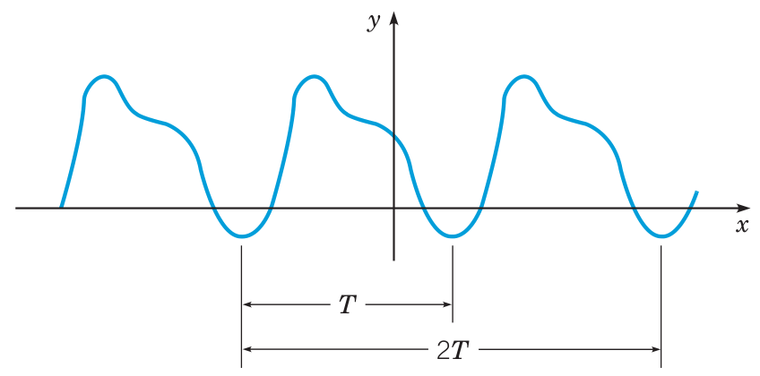
Periodic functions

• A periodic function satisfies for some constant period .
• Trig functions are periodic with period . Fourier Series are also periodic, by default with period .
• Periods can be stretched or contracted by changing variables for some . For example if has period , then has period .
• Periodic functions are completely described by their restrictions to a single period cycle. For example and are determined by their values on the interval .

Even and odd periodic extensions It is sometimes useful to take a function defined on a half interval like and extend it to a function defined on the whole interval , and from there to all of as a periodic function with period .

Even periodic extension:

Odd periodic extension:

Fourier series can be used to approximate many other functions. These functions should be either periodic functions on , or else defined or considered only on a finite interval . (Fourier series can be shifted and scaled to accommodate intervals other than .)

Fourier series convergence

If is a function for which and are both piecewise continuous, then a Fourier series is determined which approximates .

This series converges to the exact values at points where is continuous, and converges to the average of and at points where is discontinuous.

Fourier series also converge in many other cases, for example for all functions of bounded variation, such as any difference of monotone functions.

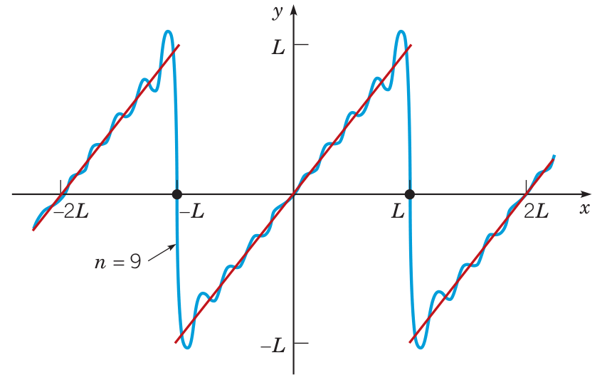
Fourier series are frequently used to reconstruct “signals” in electronics, for example, the square wave or the sawtooth wave:

Try approximating a variety of signals on this Mathlet: https://mathlets.org/mathlets/fourier-coefficients/ You can turn on the “Distance” number which quantifies the approximation error. For Signal A, using only Odd terms of the Sine series, I was able to get the error distance to . Can you beat it?

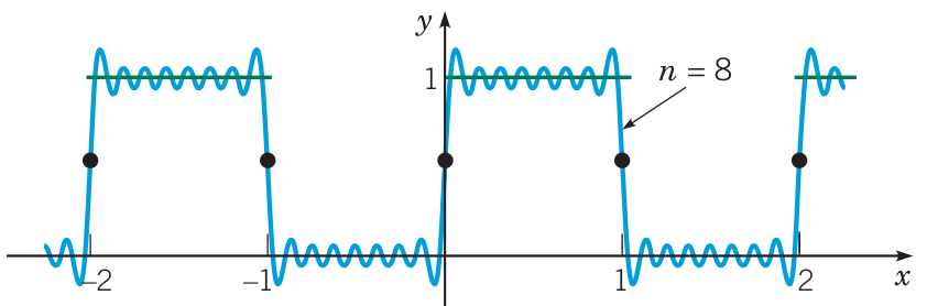
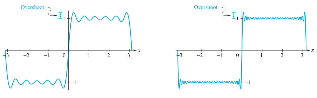
Gibb’s phenomenon

When is not continuous but only piecewise continuous, it can happen that Fourier convergence is not uniform across the interval.

The Gibb’s phenomenon is illustrated at the corners of the square wave. In this case of the Gibb’s phenomenon, overshoot remains at 9% regardless of the number of Fourier components used.

Fourier series: orthogonality relations

The terms of a Fourier series have an orthogonality property that is essential for their study. This property allows one to compute the Fourier coefficients quickly, and to show that Fourier partial sums give good approximations.

Define an inner product on pairs of functions as follows:

This product behaves like a dot product, having linearity in each input as well as symmetry:

• Symmetry:
• Sums:
• Scalars:

Two functions and are said to be orthogonal when . The norm of is defined as .

An important feature of Fourier components is that they constitute an orthogonal set of functions, as summarized in the following facts:

Another way to put this orthogonality: any pair of Fourier components and satisfies

Here and could be any of or for any .

Question 14-02

Establishing Fourier orthogonality

Show that Hint: average the trig identities for and .

Using the inner product, we can easily find the Fourier coefficients of a given function that has a Fourier series.

If , then:

For comparison: orthogonal bases and coefficients

These formulas should be compared to the basis representation of a vector using orthogonal projections.

Suppose are orthogonal vectors, and we have a linear combination representation of :

Then by taking the dot product of both sides with , we have:

Comparing to the notation of the Fourier series, and are like the vectors , the fraction is like the fraction , and the dot product is like the inner product or .

The main novelties are: (i) the even and odd components of Fourier series, and , are written separately, and (ii) Fourier components constitute an infinite list of items.

Example

Fourier coefficients for a square wave

Problem: Find the Fourier series for the square wave given by for and extended to an odd periodic function.

Solution: As an odd function, this signal will be represented by the sine series alone. So for all , while

The final Fourier series for the square wave is then:

Boundary value problems

In the next Packet we will study the wave equation and heat equation. The solution procedures will involve Fourier series, but also some of the basic ideas about boundary value problems.

The idea of a boundary value problem (BVP) is a counterpoint to the idea of an initial value problem (IVP). The BVP is to find solutions to the differential equation that pass through specified points (if their graphs are considered), or which take specified values at specified points (if their inputs only are considered in space). The ‘’ variable is used again here because it is often a spatial variable. These points are called ‘boundary values’ because of the fact that in real applications, these values are fixed known quantities taken at the boundaries of a system.

Both BVPs and IVPs are problems of determining which (if any) members of a complete family of solutions satisfy the given conditions. The BVP or IVP becomes a problem of algebra as soon as the complete family of solutions is known.

Boundary value problems are generally much more complicated than initial value problems. Given some ‘complete family of solutions,’ it is often a tricky question whether any of these solutions take on the boundary values. On the other hand, our standard theorems of existence and uniqueness often apply to yield (at least local) solutions of initial value problems. It may be hard to see why the IVP is easier than the BVP just by looking at a complete family of solutions, however.

BVP = IVP for first-order ODE

Notice! BVP = IVP in the case of first-order ODEs. Both conditions are simply the choice of a single input-output pair on the solution curve.

Example

BVP of sinusoids

Consider the ODE given by . We study the BVP given by and . The ‘boundaries’ in question are and .

We have already found the complete family of solutions to the ODE:

The first boundary condition determines , or (in the second formulation) . If we assume , then it will be enough to consider just the two options and . (Why?)

The solutions compatible with are therefore sinusoids with angular frequency that pass through the origin. At these solutions take the value . With fixed , by varying we can control the values at to a certain extent, but we are not completely free. https://www.desmos.com/calculator/sdj2z3kumw

Here is a summary of what we can do:

• If , then we must have , or else (hence everywhere)
• If , then we can solve for provided ; but if there is simply no solution.

That is a complete solution to the BVP in question.

Example

Fixing boundary, varying parameter

We can instead consider the problem from another angle. Suppose we fix the boundary data, and ask instead for the possible parameters for which nonzero solutions exist.

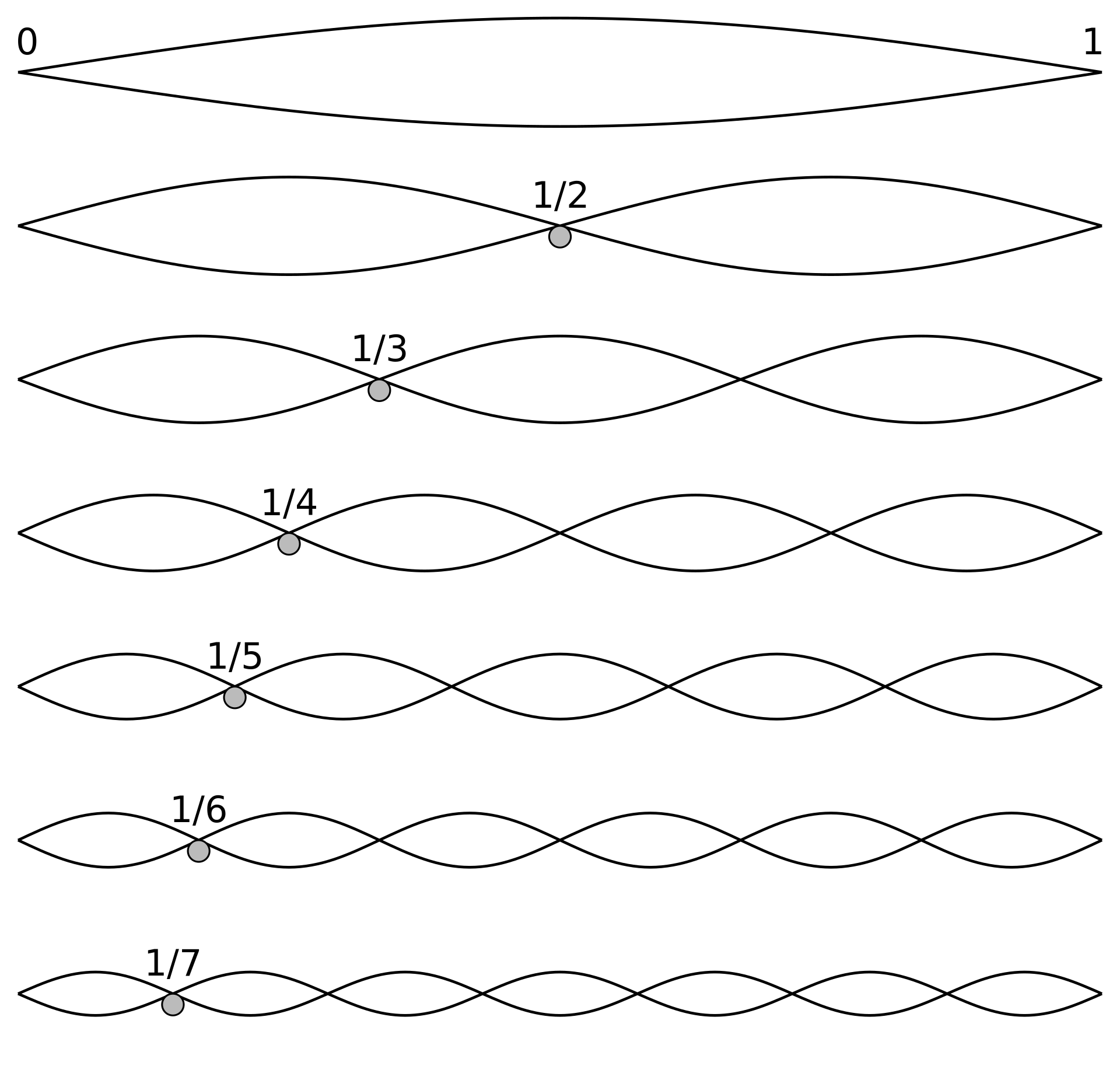
Let us fix the second boundary point at . Solutions (other than ) are only possible when . Treating as a constant, we see that nontrivial solutions exist if and only if .

In other words, the oscillation frequency must be such that the sinusoid crosses through at the boundary point . This will occur precisely when

Eigenfunctions

We have seen previously that linear differential operators determine linear differential equations of the form for any driving function .

Given a linear operator , an eigenfunction of is a function (not identically zero) satisfying for some scalar .

For example, the operator has eigenfunction that satisfies with eigenvalue . For another example, the operator has eigenfunctions that satisfy with eigenvalue .

Linearity and the concept of eigenfunction are applicable to boundary value problems when the specified boundary values are all zero. (Otherwise the sum of solutions would not be a solution.) So, for example, the BVP given by and determines a vector space of solutions. All solutions can be written as linear combinations of eigenfunctions. Infinite series of eigenfunctions also give solutions, provided they converge.

Eigenfunction solutions have a special importance in the basic theory of PDEs because many important physical PDEs specify an eigenvalue problem in each variable. This means the solutions must be eigenfunctions, but the eigenvalues themselves are free – they are not determined by the problem setup. The complete family of solutions therefore comprises the linear combinations of eigenfunctions of the BVP.

Exercise 14-01

Boundary value problem

• (a) Solve the BVP: .
• (b) Find the eigenvalues and eigenfunctions for the following BVP: .

Note carefully the primes for boundary conditions.

PDE: Wave equation

The D scalar wave equation is:

for some constant and function that depends on position and time .

If describes the vertical displacement of a rubber band, then will (to good approximation) satisfy the wave equation.

Many physical systems satisfy this equation to some degree of approximation. There are higher dimensional analogues as well. For example in D the wave equation looks like this:

Some fields that satisfy the D wave equation include:

• Density of air (sound waves).
• Each vector component of the electric or magnetic field.

An extremely important property of the wave equation is linearity. Given any two solutions and to the wave equation, any linear combination of them:

is also a solution. In physical settings, linearity implies the superposition principle that we have discussed before. In addition to its physical interest, superposition has a practical consequence: solutions to the wave equation can be broken into sums (or infinite series) of well-behaved solutions, meaning waves that are easy to describe, analyze, and visualize.

In this Packet we focus on the D scalar wave equation. We will study it from two points of view: traveling waves and standing waves. The former are sometimes just called waves, and the latter are sometimes called normal modes or simply modes for short.

These points of view correspond to wave decompositions. Traveling waves preserve a shape function as they move through space. Thinking in terms of traveling waves enables the study of energy transmission, reflections, and media interfaces. Standing waves lead to simplification of a different sort. They satisfy separation of variables which in turn leads to sinusoidal terms with nodes and peaks that are fixed in space. These sinusoids are independent of each other. They interact nicely with Fourier series.

For the rest of the section we return to the scalar wave equation, .

Traveling waves

A traveling wave is given by a function of a linear combination of space and time:

At any given fixed , the ‘shape’ of the solution across the variable is described by the same shape function , but with a horizontal shift given by .

Traveling waves satisfy the wave equation, for any shape function , when :

Exercise 14-02

Traveling waves

Verify that the functions (left-traveling wave) and (right-traveling wave) solve the wave equation. Here and are arbitrary ‘shape functions’ for these waves.

Verify that the left-traveling wave travels to the left, and the right-traveling wave travels to the right. How fast do they go? Explain.

Conversely, d’Alembert discovered an argument that essentially all solutions to are given by a sum of traveling waves, with one term traveling leftwards, and another term traveling rightwards:

Wave equation solutions are traveling waves

Suppose has all requisite partial derivatives, and it satisfies the wave equation .

Then for some and shape functions.

Derivation of d’Alembert’s solution

Let us change variables to and . Then:

and:

It follows that the wave equation is equivalent to the equation:

Now we can integrate this equation in and then in :

Here is introduced as a constant of the integration, is an antiderivative (so ), and is a constant of the integration.

Then by plugging in and we obtain:

Example

Initial shape no velocity, divides into left-moving and right-moving of same shape half size

Problem: Suppose the initial condition is given by and . How does the wave evolve?

Solution: Write the solution in the format . The initial conditions determine two equations:

The first equation implies , which we solve for and plug into the second:

Now plug this in for in the first equation to obtain , and therefore:

This is the equation of a wave with shape moving to the left superposed on a wave with shape moving to the right.

Exercise 14-03 (in class)

Divided wave

Using the solution form provided in the example, characterize the future evolution of the wave with initial condition and with Draw a picture of your answer.

Standing waves

Waves that do not travel laterally are called standing waves. This lack of lateral motion may be described mathematically by specifying a fixed shape function ; the standing wave is then described by where the amplitude depends on time, but at any given time, the shape of the wave across space (ignoring the amplitude) is . In many applied contexts, standing waves are called normal modes or simply modes.

Let us find the normal modes of the D wave equation. These are solutions of the form . From this it follows that and . The wave equation then dictates:

which implies

The left side does not depend on , and the right side does not depend on . Equality of the sides implies that both sides equal some constant . (Adding the minus sign for future convenience.)

So we end up two second order equations that are completely independent:

The solutions when are sinusoids with frequency ratio :

In the absence of boundaries, these solutions can occur with any frequency.

Free standing waves can be related to traveling waves by rewriting the product with the trig identity :

These are waves traveling with velocity , to the left and the right respectively, with the same amplitude. “Interference” of the traveling waves is equivalent to the presentation as standing waves. https://en.wikipedia.org/wiki/Standing_wave#/media/File:Waventerference.gif

Standing waves have a natural significance in the context of boundary value problems where the normal modes frequently receive a large contribution of the energy of natural vibrations. The boundary conditions have the effect of allowing only certain discrete values of , which is a kind of quantization phenomenon.

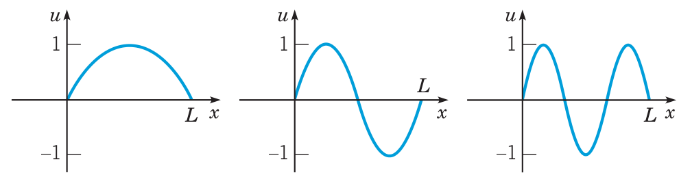
Suppose a vibrating rubber band satisfies the wave equation and boundary conditions . The natural mode solutions to this BVP are given by .

https://en.wikipedia.org/wiki/Standing_wave#/media/File:Standing_waves_on_a_string.gif

Problems due Friday 26 Apr 2024 by 11:59pm

Easier Problems

Problem 14-01

Fourier series of triangle wave

Find the Fourier series of the triangle wave in the figure: Be sure to account for the period of rather than . (You should change variables so that the wave covers one cycle on the interval in the new variable, and then change back at the very end to express your final answer.)

Problem 14-02

Full Fourier series with rescaling, even and odd parts

Compute the Fourier series for the function defined on the interval .

You should first change to a new independent variable for which that interval corresponds to the interval , and change back at the end.

Problem 14-03 = Exercise 14-02

Traveling waves

Verify that the functions (left-traveling wave) and (right-traveling wave) solve the wave equation. Here and are arbitrary ‘shape functions’ for these waves. Verify that the left-traveling wave travels to the left, and the right-traveling wave travels to the right. How fast do they go?

Harder Problems

Problem 14-04

Fourier series can teach us about

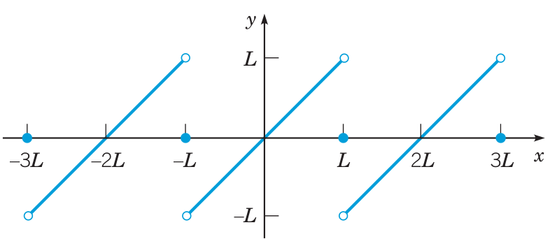
• (a) Compute the Fourier series of the following sawtooth wave with :
• (b) Evaluate your Fourier series at to establish Leibniz’s famous formula:

• (c) Find a similar series expression for using your solution to Problem 14-01.

Problem 14-05

Fourier series can solve initial value problems

For this problem, you should solve the given ODE by plugging in a generic Fourier series and solving for the coefficients. Fourier coefficients are uniquely determined because Fourier terms are orthogonal.

• (a)
• (b) , where is the triangle wave in Problem 14-01. (Substitute the Fourier series you found for .)

Problem 14-06

Plucked band

A rubber band fixed at and is plucked by stretching the center point to a height of and releasing it. At the point of release, the band shape is an isosceles triangle with base width and height .

Find the function that describes the future evolution of the band, written as a sum of normal modes. Is a standing wave? (If yes, prove it; if no, demonstrate that it cannot be one.)

You should assume the band satisfies the BVP given by and for all . To find your solution , first write down the initial shape function at the moment of release, and then compute its Fourier series in . (Review and modify your work in Problem 14-01.) Any solution is a sum of normal modes. Using the theory of orthogonality of Fourier terms, solve for the coefficients of the normal modes in your solution.