Theory

Theory 1

Random variable

A random variable (RV) $X$ on a probability space $(S,ℱ,P)$ is a function $X:S\to ℝ$.

So $X$ assigns to each outcome a number.

Note: The word ‘variable’ indicates that an RV outputs numbers.

Random variables can be formed from other random variables using mathematical operations on the output numbers.

Given random variables $X$ and $Y$, we can form these new ones:

$$\frac{1}{2}(X+Y),X\cdot Y,\cos X,X^2,\text{etc.}$$

Suppose $s\in S$ is some particular outcome. Then, for example, $(X+Y)(s)$ is by definition $X(s)+Y(s)$.

---

Random variables determine events.

• Given $a\in ℝ$, the event “$X=a$” is equal to the set $X^{-1}(a)$
• That is: the set of outcomes mapped to $a$ by $X$
• That is: the event “$X$ took the value $a$”

Such events have probabilities. We write them like this:

$$P[X=a]\gg \gg P[X^{-1}(a)]$$

This generalized to events where $X$ lies in some range or set, for example:

$$P[a\le X<b],P[X\in \{\mathrm{2,4,5,6,9}\}]$$

---

The axioms of probability translate into rules for these events.

For example, additivity leads to:

$$P[X<0]+P[X=0]+P[0<X\le 3]+P[3<X]=1$$

---

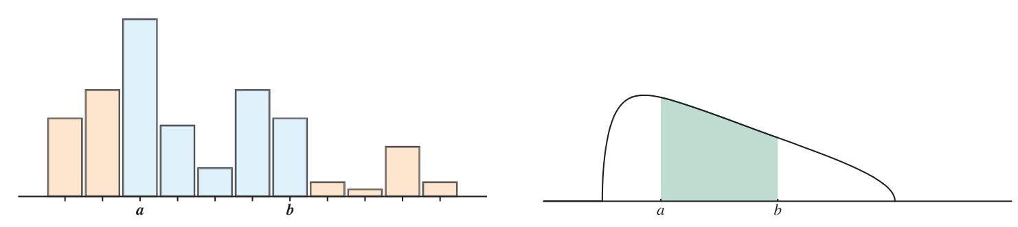
A discrete random variable has probability concentrated at a discrete set of real numbers.

• A ‘discrete set’ means finite or countably infinite.
• The distribution of probability is recorded using a probability mass function (PMF) that assigns probabilities to each of the discrete real numbers.
• Numbers with nonzero probability are called possible values.

PMF

The PMF function $P_X(k)$, for $X$ a discrete RV, is defined by:

$$P_X(k)=P[X=k]$$

A continuous random variable has probability spread out over the space of real numbers.

• The distribution of probability is recorded using a probability density function (PDF) which is integrated over intervals to determine probabilities.

PDF

The PDF function for $Y$ (a CRV) is written $f_Y(x)$ for $x\in ℝ$, and probabilities are calculated like this:

$$P[a\le Y\le b]={\int }_a^b{f}_Y(x)dx$$

---

For any RV, whether discrete or continuous, the distribution of probability is encoded by a function:

CDF

The cumulative distribution function (CDF) for a random variable $X$ is defined for all $x\in ℝ$ by: $F_X(x)=P[X\le x]$

Notes:

• Sometimes the relation to $X$ is omitted and one sees just “$F(x)$.”
• Sometimes the CDF is called, simply, “the distribution function” because:

The CDF works for a discrete, continuous, or mixed RV

• PMF is for discrete only
• PDF is for continuous only
• CDF covers both and covers mixed RVs

---

The CDF of a discrete RV is always a stepwise increasing function. At each step up, the jump size matches the PMF value there.

From this graph of $F_X(x)$:

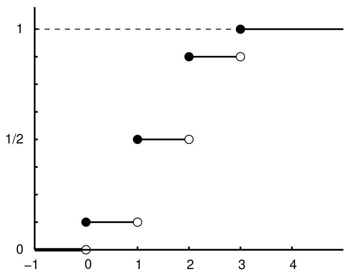
we can infer the PMF values based on the jump sizes:

$P_X(-1)$	$P_X(0)$	$P_X(1)$	$P_X(2)$	$P_X(3)$	$P_X(4)$
$0$	$1/8$	$3/8$	$3/8$	$1/8$	$0$

---

For a discrete RV, the CDF and the PMF can be calculated from each other using formulas.

PMF from CDF

Given a PMF $P_X(x)$, the CDF is determined by:

$$F_X(x)=\sum _{k_i\le x}{P}_X(k_i)$$

where $\{k_1,k_2,\dots \}$ is the set of possible values of $X$.