Theory

Theory 1 - Poisson variable

Poisson variable

A random variable $X$ is Poisson, written $X\sim \mathrm{Pois}(\alpha )$, when $X$ counts the number of “arrivals” in a fixed “window.” It is applicable when:

• The arrivals come at a constant average rate.
• The arrivals are independent of each other.

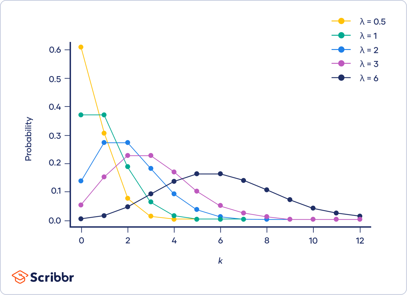
Poisson PMF:

$$P_X(k)=e^{-\alpha }\frac{{\alpha }^k}{k!}$$

The “window rate” $\alpha$ must be computed from the “background rate” $\lambda$ using the window size.

A Poisson variable is comparable with a binomial variable. Both count the occurrences of some “arrivals” over some “space of opportunity.”

• The binomial opportunity is a set of $n$ repetitions of a trial.
• The Poisson opportunity is a continuous interval of time.

In the binomial case, success occurs at some rate $p$, since $p=P[A]$ where $A$ is the success event.

In the Poisson case, arrivals occur at some rate $\alpha$.

---

---

The Poisson distribution is actually the limit of binomial distributions by taking $n\to \infty$ while $np$ remains fixed, so $p\to 0$ in perfect balance with $n\to \infty$.

Fix $\alpha$ and define $p_n=\alpha /n$. (So $p$ is computed to ensure the average rate $np$ does not change.) Let $X_n\sim \mathrm{Bin}(n,p_n)$ and let $Y_{\alpha }\sim \mathrm{Pois}(\alpha )$. Then for any $k\in \mathbb{N}$:

$$P_{X_n}(k)\to P_{Y_{\alpha }}(k)\text{as }n\to \infty$$

For example, let $X_n\sim \mathrm{Bin}(n,p_n)$, so with $p_n=\frac{3}{n}$, and look at $P_{X_n}(1)$ as $n\to \infty$:

$$\begin{array}{c}{P}_{X_n}(1)\gg \gg \left(\genfrac{}{}{0px}{}{n}{1}\right){\left(\frac{3}{n}\right)}^1{(1-\frac{3}{n})}^{n-1}\\ \\ \gg \gg 3{(1-\frac{3}{n})}^{n-1}⟶3e^{-3}\text{as}n\to \infty \end{array}$$

Interpretation - Binomial model of rare events

Let us interpret the assumptions of this limit. For $n$ large but $p$ small such that $\alpha =np$ remains moderate, the binomial distribution describes a large number of trials, a low probability of success per trial, but a moderate total count of successes.

This setup describes a physical system with a large number of parts that may activate, but each part is unlikely to activate; and yet the number of parts is so large that the total number of arrivals is still moderate.

Theory 2 - Poisson limit of binomial

Extra - Derivation of binomial limit to Poisson

Consider a random variable $X\sim \mathrm{Bin}(n,p)$, and suppose $n$ is very large.

Suppose also that $p$ is very small, such that $E[X]=np$ is not very large, but the extremes of $n$ and $p$ counteract each other. (Notice that then $npq$ will not be large so the normal approximation does not apply.) In this case, the binomial PMF can be approximated using a factor of $e^{-np}$. Consider the following rearrangement of the binomial PMF:

$$\begin{array}{c}{P}_X(k)\gg \gg \left(\genfrac{}{}{0px}{}{n}{k}\right)p^k{q}^{n-k}\\ \\ \gg \gg \frac{n(n-1)\cdots (n-k+1)}{k!}{p}^k{(1-p)}^n\frac{1}{q^k}\\ \\ \gg \gg {(1-p)}^n\frac{{(np)}^k}{k!}[\frac{n}{n}\cdot \frac{n-1}{n}\cdot \frac{n-2}{n}\cdots \frac{n-k+1}{n}]\frac{1}{q^k}\end{array}$$

Since $n$ is very large, the factor in brackets is approximately $1$, and since $p$ is very small, the last factor of $1/q^k$ is also approximately 1 (provided we consider $k$ small compared to $n$). So we have:

$$P_X(k)\approx {(1-p)}^n\frac{{(np)}^k}{k!}.$$

Write $\alpha =np$, a moderate number, to find:

$$P_X(k)\approx {(1-\frac{\alpha }{n})}^n\frac{{\alpha }^k}{k!}.$$

Here at last we find $e^{-\alpha }$, since ${(1-\frac{\alpha }{n})}^n\to e^{-\alpha }$ as $n\to \infty$. So as $n\to \infty$:

$$P_X(k)\approx e^{-\alpha }\frac{{\alpha }^k}{k!}.$$

Theory 3 - Divisibility

Extra - Divisibility

Consider a sequence of increasing $n$ with decreasing $p$ such that $\alpha =np$ is held fixed. For example, let $n=\mathrm{1,2,3},\dots$ while $p=\frac{\alpha }{n}$.

Think of this process as increasing the number of causal agents represented: group the agents together into $n$ bunches, and consider the odds that such a bunch activates. (For the call center, a bunch is a group of users; for radioactive decay, a bunch is a unit of mass of Uranium atoms.)

As $n$ doubles, we imagine the number of agents per bunch to drop by half. (For the call center, we divide a group in half, so twice as many groups but half the odds of one group making a call; for the Uranium, we divide a chunk of mass in half, getting twice as many portions with half the odds of a decay occurring in each portion.

This process is formally called division of a distribution, and the fact that the Poisson distribution arises as the limit of such division means that it is infinitely divisible.

Theory 4 - Poisson approximation

Extra - Theorem: Poisson approximation of the binomial

Suppose $X\sim \mathrm{Bin}(n,p)$ and $Y\sim \mathrm{Pois}(np)$. Then:

$$|P_X(k)-P_Y(k)|\le n{p}^2$$

for any $k\in \mathbb{N}$.

In consequence of this theorem, a Poisson distribution may be used to approximate the probabilities of a binomial distribution for large $n$ when it is impracticable (even for a computer) to calculate large binomial coefficients.

The theorem shows that the Poisson approximation is appropriate when $np$ is a moderate number while $n{p}^2$ is a small number.