Theory

Theory 1

Joint distributions describe the probabilities of events associated with multiple random variables simultaneously.

In this course we consider only two variables at a time, typically called $X$ and $Y$. It is easy to extend this theory to vectors of $n$ random variables.

Joint PMF and joint PDF

Discrete joint PMF:

$$P_{X,Y}(x,y)=P[X=x,Y=y]$$

Continuous joint PDF:

$$f_{X,Y}(x,y)=\text{density at}(x,y)$$

Probabilities of events: Discrete case If $B\subset {ℝ}^2$ is a set of points in the plane, then an event $ℬ$ is formed by the set of all outcomes $s$ mapped by $X$ and $Y$ to points in $B$:

$$ℬ=\{s\in S|(X(s),Y(s))\in B\}$$

The probabilities of such events can be measured using the joint PMF:

$$P[(X,Y)\in B]=P[ℬ]=\sum _{(x,y)\in B}{P}_{X,Y}(x,y)$$

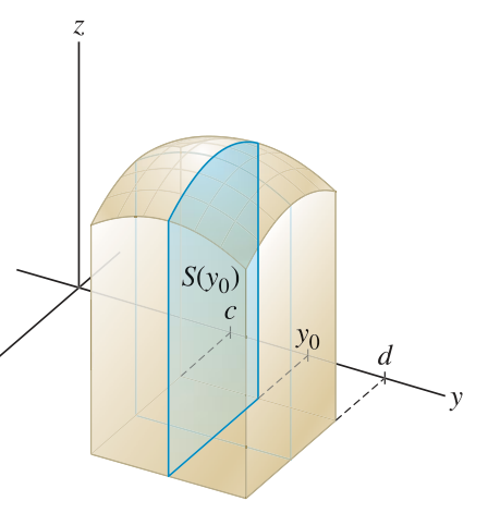
Probabilities of events: Continuous case Let $𝒱=[a,b]\times [c,d]\subset {ℝ}^2$ be the rectangular region defined by $(x,y)\in {ℝ}^2$ such that $a\le x\le b$ and $c\le y\le d$. Then:

$$P[(x,y)\in 𝒱]=P[a\le X\le b,c\le Y\le d]={\int }_c^d{\int }_a^b{f}_{X,Y}(x,y)dxdy$$

For more general regions $𝒱\subset {ℝ}^2$:

$$P[(X,Y)\in 𝒱]={\iint }_{𝒱}{f}_{X,Y}(x,y)dA$$

---

The existence of a variable $Y$ does not change the theory for a variable $X$ considered by itself.

However, it is possible to relate the theory for $X$ to the theory for $(X,Y)$, in various ways.

The simplest relationship is the marginal distribution for $X$, which is merely the distribution of $X$ itself, considered as a single random variable, but in a context where it is derived from the joint distribution for $(X,Y)$.

Marginal PMF, marginal PDF

Marginal distributions are obtained from joint distributions by summing the probabilities over all possibilities of the other variable.

Discrete marginal PMF:

$$\begin{array}{cc}{P}_X(x)& =\sum _y{P}_{X,Y}(x,y)\\ & \\ P_Y(y)& =\sum _x{P}_{X,Y}(x,y)\end{array}$$

Continuous marginal PMF:

$$\begin{array}{cc}{f}_X(x)& ={\int }_{-\infty }^{+\infty }{f}_{X,Y}(x,y)dy\\ & \\ f_Y(y)& ={\int }_{-\infty }^{+\infty }{f}_{X,Y}(x,y)dx\end{array}$$

---

Infinitesimal method

Suppose $X$ has density $f_X(x)$ that is continuous at $x_0$. Then for infinitesimal $dx$:

$$P[x_0<X\le x_0+dx]=f_X(x)dx$$

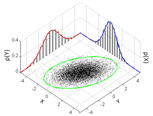
Suppose $X$ and $Y$ have joint density $f_{X,Y}(x,y)$ that is continuous at $(x_0,y_0)$. Then for infinitesimal $dx,dy$:

$$P[x_0<X\le x_0+dx,y_0<Y\le y_0+dy]=f_{X,Y}(x_0,y_0)dxdy$$

Joint densities depend on coordinates

The density $f_{X,Y}(x,y)$ in these integration formulas depends on the way $X$ and $Y$ act as Cartesian coordinates and determine differential areas $dxdy$ as little rectangles.

To find a density $f_{R,\mathrm{\Theta }}(r,\theta )$ in polar coordinates, for example, it is not enough to solve for $x(r,\theta )$ and $y(r,\theta )$ and plug into $f_{X,Y}$!

Instead, we must consider the differential area $dxdy$ vs. $drd\theta$. We find that $dxdy=rdrd\theta$.

As an example, the density of the uniform distribution on the unit disk is $f_{R,\mathrm{\Theta }}={\displaystyle \frac{r}{\pi }}$, which is not constant as a function of $r$ and $\theta$.

Extra - Joint densities may not exist

It is not always possible to form a joint PDF $f_{X,Y}$ from any two continuous RVs $X$ and $Y$.

For example, if $X=Y$, then $(X,Y)$ cannot have a joint PDF, since $P[X=Y]=1$ but the integral over the region $X=Y$ will always be 0. (The area of a line is zero.)

Theory 2

Joint CDF

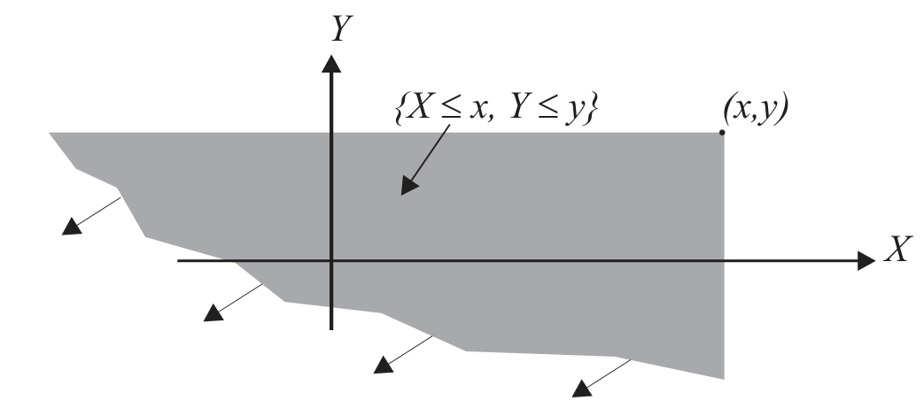
The joint CDF of $X$ and $Y$ is defined by:

$$F_{X,Y}(x,y)=P[X\le x,Y\le y]$$

We can relate the joint CDF to the joint PDF using integration:

$$F_{X,Y}(x,y)={\int }_{-\infty }^y{\int }_{-\infty }^x{f}_{X,Y}(s,t)dsdt$$

Conversely, if $X$ and $Y$ have a continuous joint PDF $f_{X,Y}(x,y)$ that is also differentiable, we can obtain the PDF from the CDF using partial derivatives:

$$f_{X,Y}(x,y)=\frac{{\partial }^2}{\partial x\partial y}{F}_{X,Y}(x,y)$$

---

There is also a marginal CDF that is computed using a limit:

$$F_X(x)=\underset{y\to +\infty }{\lim }{F}_{X,Y}(x,y)$$

This could also be written, somewhat abusing notation, as $F_X(x)=F_{X,Y}(x,+\infty )$.