W05 Notes

Poisson process

01 Theory - Poisson variable

Theory 1 - Poisson variable

Poisson variable

A random variable $X$ is Poisson, written $X\sim \mathrm{Pois}(\alpha )$, when $X$ counts the number of “arrivals” in a fixed “window.” It is applicable when:

• The arrivals come at a constant average rate.
• The arrivals are independent of each other.

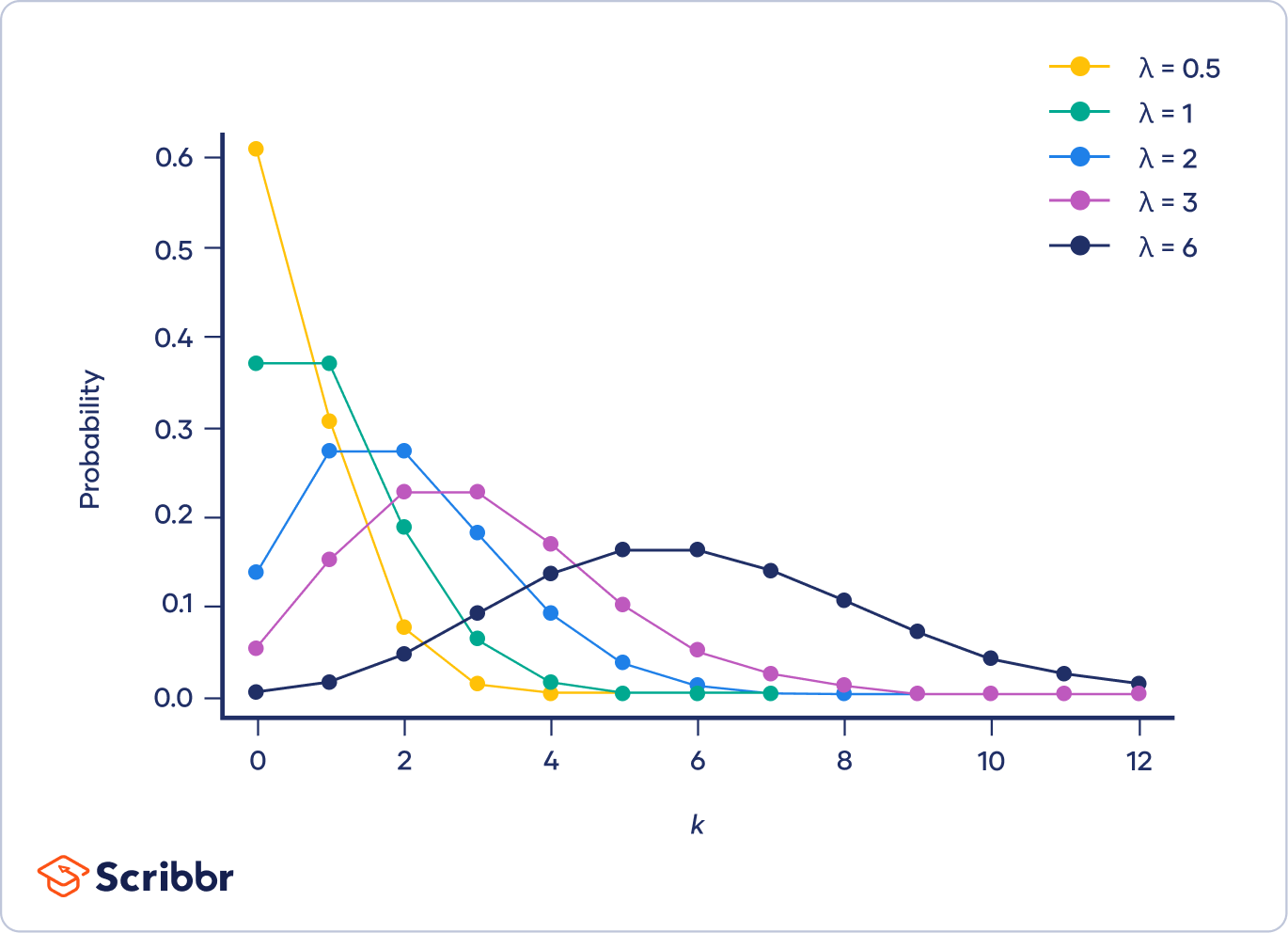
Poisson PMF:

$$P_X(k)=e^{-\alpha }\frac{{\alpha }^k}{k!}$$

The “window rate” $\alpha$ must be computed from the “background rate” $\lambda$ using the window size.

A Poisson variable is comparable with a binomial variable. Both count the occurrences of some “arrivals” over some “space of opportunity.”

• The binomial opportunity is a set of $n$ repetitions of a trial.
• The Poisson opportunity is a continuous interval of time.

In the binomial case, success occurs at some rate $p$, since $p=P[A]$ where $A$ is the success event.

In the Poisson case, arrivals occur at some rate $\alpha$.

---

---

The Poisson distribution is actually the limit of binomial distributions by taking $n\to \infty$ while $np$ remains fixed, so $p\to 0$ in perfect balance with $n\to \infty$.

Fix $\alpha$ and define $p_n=\alpha /n$. (So $p$ is computed to ensure the average rate $np$ does not change.) Let $X_n\sim \mathrm{Bin}(n,p_n)$ and let $Y_{\alpha }\sim \mathrm{Pois}(\alpha )$. Then for any $k\in \mathbb{N}$:

$$P_{X_n}(k)\to P_{Y_{\alpha }}(k)\text{as }n\to \infty$$

For example, let $X_n\sim \mathrm{Bin}(n,p_n)$, so with $p_n=\frac{3}{n}$, and look at $P_{X_n}(1)$ as $n\to \infty$:

$$\begin{array}{c}{P}_{X_n}(1)\gg \gg \left(\genfrac{}{}{0px}{}{n}{1}\right){\left(\frac{3}{n}\right)}^1{(1-\frac{3}{n})}^{n-1}\\ \\ \gg \gg 3{(1-\frac{3}{n})}^{n-1}⟶3e^{-3}\text{as}n\to \infty \end{array}$$

Interpretation - Binomial model of rare events

Let us interpret the assumptions of this limit. For $n$ large but $p$ small such that $\alpha =np$ remains moderate, the binomial distribution describes a large number of trials, a low probability of success per trial, but a moderate total count of successes.

This setup describes a physical system with a large number of parts that may activate, but each part is unlikely to activate; and yet the number of parts is so large that the total number of arrivals is still moderate.

Link to original

02 Illustration

Example - Arrivals at a post office

Arrivals at a post office

Client arrivals at a post office are modelled well using a Poisson variable.

Each potential client has a very low and independent chance of coming to the post office, but there are many thousands of potential clients, so the arrivals at the office actually come in moderate number.

Suppose the average rate is 5 clients per hour.

(a) Find the probability that nobody comes in the first 10 minutes of opening. (The cashier is considering being late by 10 minutes to run an errand on the way to work.)

(b) Find the probability that 5 clients come in the first hour. (I.e. the average is achieved.)

(c) Find the probability that 9 clients come in the first two hours.

Solution

(a)

Expect $5/6$ clients every 10 minutes. Therefore, let $X\sim \mathrm{Pois}(5/6)$. Seek $P_X(0)$ as the answer.

PMF:

$$P_X(k)=e^{-5/6}\frac{{(5/6)}^k}{k!}$$

Insert data and compute:

$$P_X(0)\gg \gg e^{-5/6}\gg \gg \approx 0.435$$

---

(b)

Rate is already correct. Let $X\sim \mathrm{Pois}(5)$.

PMF:

$$P_X(5)=e^{-5}\frac{5^5}{5!}\gg \gg \approx 0.175$$

---

(c)

Expect 10 clients every 2 hours. Therefore let $X\sim \mathrm{Pois}(10)$.

PMF:

$$P_X(9)\gg \gg e^{-10}\frac{{10}^9}{9!}\gg \gg \approx 0.125$$

Notice that 0.125 is smaller than 0.175.

Link to original

Example - Random leukemia?

Random leukemia?

Suppose the rate of leukemia in a random population is expected to be 8.3 cases per million.

Suppose a given town of 150,000 residents has 12 cases. Is that suspicious?

(Compute the probability of 12 or more cases assuming a Poisson distribution.)

Solution

The expected case rate for 150,000 residents is:

$$(1.5\times {10}^5\mathrm{persons})\cdot \frac{8.3\mathrm{cases}}{1\times {10}^6\mathrm{persons}}\gg \gg 1.245$$

Therefore, with a “window” of 150,000, the case rate should be $\alpha =1.245$. Set $X\sim \mathrm{Pois}(1.245)$.

Now compute:

$$\begin{array}{c}P[X\ge 12]=\sum _{k=12}^{\infty }{P}_X(k)\\ \\ \gg \gg 1-\sum _{k=0}^{11}{e}^{-1.245}\frac{{(1.245)}^k}{k!}\gg \gg 9.12\times {10}^{-9}\end{array}$$

Therefore the observed case rate is highly suspicious!

Link to original

Example - Radioactive decay is Poisson

Radioactive decay is Poisson

Consider a macroscopic sample of Uranium.

Each atom decays independently of the others, and the likelihood of a single atom popping off is very low; but the product of this likelihood by the total number of atoms is a moderate number.

So there is some constant average rate of atoms in the sample popping off, and the number of pops per minute follows a Poisson distribution.

Link to original

Example - Typos per page

Typos per page

A draft of a textbook has an average of 6 typos per page.

What is the probability that a randomly chosen page has $\ge 4$ typos?

(Answer: 0.849. Hint: study the complementary event.)

Link to original

03 Theory - Poisson limit of binomial

Theory 2 - Poisson limit of binomial

Extra - Derivation of binomial limit to Poisson

Consider a random variable $X\sim \mathrm{Bin}(n,p)$, and suppose $n$ is very large.

Suppose also that $p$ is very small, such that $E[X]=np$ is not very large, but the extremes of $n$ and $p$ counteract each other. (Notice that then $npq$ will not be large so the normal approximation does not apply.) In this case, the binomial PMF can be approximated using a factor of $e^{-np}$. Consider the following rearrangement of the binomial PMF:

$$\begin{array}{c}{P}_X(k)\gg \gg \left(\genfrac{}{}{0px}{}{n}{k}\right)p^k{q}^{n-k}\\ \\ \gg \gg \frac{n(n-1)\cdots (n-k+1)}{k!}{p}^k{(1-p)}^n\frac{1}{q^k}\\ \\ \gg \gg {(1-p)}^n\frac{{(np)}^k}{k!}[\frac{n}{n}\cdot \frac{n-1}{n}\cdot \frac{n-2}{n}\cdots \frac{n-k+1}{n}]\frac{1}{q^k}\end{array}$$

Since $n$ is very large, the factor in brackets is approximately $1$, and since $p$ is very small, the last factor of $1/q^k$ is also approximately 1 (provided we consider $k$ small compared to $n$). So we have:

$$P_X(k)\approx {(1-p)}^n\frac{{(np)}^k}{k!}.$$

Write $\alpha =np$, a moderate number, to find:

$$P_X(k)\approx {(1-\frac{\alpha }{n})}^n\frac{{\alpha }^k}{k!}.$$

Here at last we find $e^{-\alpha }$, since ${(1-\frac{\alpha }{n})}^n\to e^{-\alpha }$ as $n\to \infty$. So as $n\to \infty$:

$$P_X(k)\approx e^{-\alpha }\frac{{\alpha }^k}{k!}.$$

Link to original

04 Theory - Poisson expected value

02

Expectation of Poisson

Derive the formula $E[X]=\alpha$ for a Poisson variable $X\sim \mathrm{Pois}(\alpha )$.

Solution

Solutions - 5130-02

PMF of a Poisson distribution:

$$P_X(k)=e^{-\alpha }\frac{{\alpha }^k}{k!}$$

Expected value:

$$\begin{array}{c}E[X]=\sum _{k=0}^{\infty }k{P}_X(k)\\ \\ \gg \gg \sum _{k=0}^{\infty }{e}^{-\alpha }\frac{{\alpha }^k}{(k-1)!}\\ \\ \gg \gg \alpha e^{-\alpha }\sum _{k=0}^{\infty }\frac{{\alpha }^{k-1}}{(k-1)!}\\ \\ \gg \gg \alpha e^{-\alpha }{e}^{\alpha }\gg \gg \alpha \end{array}$$Link to original

Link to original

05 Theory

Theory 1

Exponential variable

A random variable $X$ is exponential, written $X\sim \text{Exp}(\lambda )$, when $X$ measures the wait time until first arrival in a Poisson process with rate $\lambda$.

Exponential PDF:

$$f_X(t)=\{\begin{array}{cc}\lambda e^{-\lambda t}& t\ge 0\\ 0& t<0\end{array}$$

• Poisson is continuous analog of binomial
• Exponential is continuous analog of geometric

---

Notice the coefficient $\lambda$ in $f_X$. This ensures $P[-\infty \le X\le \infty ]=1$:

$${\int }_0^{\infty }{e}^{-\lambda t}dt\gg \gg -{\lambda }^{-1}(e^{-\lambda \cdot \infty }-1)\gg \gg {\lambda }^{-1}$$

---

Notice the “tail probability” is a simple exponential decay:

$$P[X>t]=e^{-\lambda t}$$

(Compute an improper integral to verify this.)

---

Erlang variable

A random variable $X$ is Erlang, written $X\sim \mathrm{Erlang}(\ell ,\lambda )$, when $X$ measures the wait time until ${\ell }^{\text{th}}$ arrival in a Poisson process with rate $\lambda$.

Erlang PDF:

$$f_X(t)=\frac{{\lambda }^{\ell }}{(\ell -1)!}{t}^{\ell -1}{e}^{-\lambda t}$$

• Erlang is continuous analog of Pascal

Link to original

06 Illustration

Example - Earthquake wait time

Earthquake wait time

Suppose the San Andreas fault produces major earthquakes modeled by a Poisson process, with an average of 1 major earthquake every 100 years.

(a) What is the probability that there will not be a major earthquake in the next 20 years?

(b) What is the probability that three earthquakes will strike within the next 20 years?

Solution

(a)

Since the average wait time is 100 years, we set $\lambda =0.01$ earthquakes per year. Set $X\sim \mathrm{Exp}(0.01)$ and compute:

$$P[X>20]=e^{-\lambda \cdot 20}\gg \gg e^{-0.01\cdot 20}\gg \gg \approx 0.82$$

---

(b)

The same Poisson process has the same $\lambda =0.01$ earthquakes per year. Set $X\sim \mathrm{Erlang}(\mathrm{3,0.01})$, so:

$$\begin{array}{c}{f}_X(t)=\frac{{\lambda }^{\ell }}{(\ell -1)!}{t}^{\ell -1}{e}^{-\lambda t}\\ \\ \gg \gg \frac{{(0.01)}^3}{(3-1)!}{t}^{3-1}{e}^{-0.01\cdot t}\gg \gg \frac{{10}^{-6}}{2}{t}^2{e}^{-0.01\cdot t}\end{array}$$

Now compute:

$$\begin{array}{c}P[X\le 20]={\int }_0^{20}{f}_X(x)dx\\ \\ \gg \gg {\int }_0^{20}\frac{{10}^{-6}}{2}{t}^2{e}^{-0.01\cdot t}dt\gg \gg \approx 0.00115\end{array}$$Link to original

07 Theory

Theory 2

The memoryless distribution is exponential

The exponential distribution is memoryless. This means that knowledge that an event has not yet occurred does not affect the probability of its occurring in future time intervals:

$$P[X>t+s|X>t]=P[X>s].$$

This is easily checked using the PDF:

$$e^{-\lambda (t+s)}/e^{-\lambda t}=e^{-\lambda s}$$

No other continuous distribution is memoryless. This means any other (continuous) memoryless distribution agrees in probability with the exponential distribution. The reason is that the memoryless property can be rewritten as $P[X>t+s]=P[X>t]P[X>s]$. Consider $P[X>x]$ as a function of $x$, and notice that this function converts sums into products. Only the exponential function can do this.

The geometric distribution is the discrete memoryless distribution.

$$\begin{array}{c}P[X>n]\gg \gg \sum _{k=n+1}^{\infty }{q}^{k-1}p\gg \gg q^{n}p(1+q+q^2+\dots )\\ \\ \gg \gg q^n\frac{p}{1-q}\gg \gg q^n\end{array}$$

and by substituting $n+k$, we also know $P[X>n+k]=q^{n+k}$.

Then:

$$\begin{array}{c}P[X=n+k|X>n]\gg \gg \frac{P[X=n+k]}{P[X>n]}\gg \gg \frac{q^{n+k-1}p}{q^n}\\ \\ \gg \gg q^{k-1}p\gg \gg P[X=k]\end{array}$$

Link to original

Derived random variables

08 Theory

Theory 1

By composing any function $g:ℝ\to ℝ$ with a random variable $X:S\to ℝ$ we obtain a new random variable $g\circ X$. This one is called a derived random variable.

Notation

The derived random variable $g\circ X$ may be written “$g(X)$”.

Expectation of derived variables

Discrete case:

$$E[g(X)]=\sum _{k}g(k)\cdot P_X(k)$$

(Here the sum is over all possible values $k$ of $X$, i.e. where $P_X(k)\ne 0$.)

Continuous case:

$$E[g(X)]={\int }_{-\infty }^{+\infty }g(x)\cdot f_X(x)dx$$

Notice: when applied to outcome $s\in S$:

• $k$ is the output of $X$
• $g(k)$ is the output of $g\circ X$

The proofs of these formulas are tricky because we must relate the PDF or PMF of $X$ to that of $g(X)$.

Proof - Discrete case - Expectation of derived variable

$$\begin{array}{cc}E[g(X)]& =\sum _{y}y\cdot P_{g(X)}(y)\\ & \\ & =\sum _{y}y\cdot \sum _{k\in g^{-1}(y)}{P}_X(k)\\ & \\ & =\sum _y\sum _{k\in g^{-1}(y)}g(k)\cdot P_X(k)\\ & \\ & =\sum _{k}g(k)\cdot P_X(k)\end{array}$$

---

Linearity of expectation

For constants $a$ and $b$:

$$E[aX+b]=aE[X]+b$$

For any $X$ and $Y$ on the same probability model:

$$E[X+Y]=E[X]+E[Y]$$

Exercise - Linearity of expectation

Using the definition of expectation, verify both linearity formulas for the discrete case.

Be careful!

Usually $E[g(X)]\ne g(E[X])$.

For example, usually $E[X\cdot X]\ne E[X]\cdot E[X]$.

We distribute $E$ over sums but not products (unless the factors are independent).

---

Variance squares the scale factor

For constants $a$ and $b$:

$$\mathrm{Var}[aX+b]=a^2\mathrm{Var}[X]$$

Thus variance ignores the offset and squares the scale factor. It is not linear!

Proof - Variance squares the scale factor

$$\begin{array}{cc}\mathrm{Var}[aX+b]& =E[{(aX+b-E[aX+b])}^2]\\ & \\ & =E[{(aX+b-a{\mu }_X-b)}^2]\\ & \\ & =E[{(aX-a{\mu }_X)}^2]\\ & \\ & =E[a^2{(X-{\mu }_X)}^2]\\ & \\ & =a^{2}E[{(X-{\mu }_X)}^2]\\ & \\ & =a^2\mathrm{Var}[X]\end{array}$$

---

Extra - Moments

The $n^{\text{th}}$ moment of $X$ is defined as the expectation of $X^n$:

Discrete case:

$$E[X^n]=\sum _k{k}^n\cdot p(k)$$

Continuous case:

$$E[X^n]={\int }_{-\infty }^{+\infty }{x}^n\cdot f(x)dx$$

A central moment of $X$ is a moment of the variable $X-E[X]$:

$$E[(X-E[X]{)}^n]$$

The data of all the moments collectively determines the probability distribution. This fact can be very useful! In this way moments give an analogue of a series representation, and are sometimes more useful than the PDF or CDF for encoding the distribution.

Link to original

09 Illustration

Example - Function given by chart

Expectation of function on RV given by chart

Suppose that $g:ℝ\to ℝ$ in such a way that $g:1\mapsto 4$ and $g:2\mapsto 1$ and $g:3\mapsto 87$ and no other values are mapped to $4,1,87$. Define $Y=g(X)$.

$X:$	1	2	3
$P_X(k):$	$1/7$	$2/7$	$4/7$
$Y:$	4	1	87

Then:

$$E[X]=1\cdot \frac{1}{7}+2\cdot \frac{2}{7}+3\cdot \frac{4}{7}\gg \gg \frac{17}{7}$$

And:

$$E[Y]=4\cdot \frac{1}{7}+1\cdot \frac{2}{7}+87\cdot \frac{4}{7}\gg \gg \frac{354}{7}$$

Therefore:

$$E[5X+2Y+3]\gg \gg 5\cdot \frac{17}{7}+2\cdot \frac{354}{7}+3\gg \gg \frac{814}{7}$$ Link to original

Example - PMF across many-to-one function

PMF through many-to-one function

Suppose the PMF of $X$ is given by:

$$P_X(x)=\{\begin{array}{cc}0.2& x=-1\\ 0.4& x=0\\ 0.4& x=+1\\ 0& \text{else}\end{array}$$

Now suppose $Y=|X|$. That is to say, $Y=g(X)$ and $g(X)=|X|$.

What is the PMF of $Y$?

Solution

Notice that $g(+1)=1$ and $g(-1)=1$. So $P_X(+1)$ and $P_X(-1)$ are combined into $P_Y(1)$:

$$P_Y(y)=\{\begin{array}{cc}0.4& y=0\\ 0.6& y=1\\ 0& \text{else}\end{array}$$ Link to original

Example - Average pay raise

Average pay raise

Suppose the average salary at Company A is $52,000. Each employee is given a 3% raise and a $2000 bonus. What is the average salary now?

Solution

Let $X$ be a random variable indicating the starting salary of each employee.

Then $Y=g(X)=(1.03)X+2000$ is a random variable giving the new salary of each employee.

We can calculate the expectation by linearity:

$$\begin{array}{c}E[Y]=E[g(X)]\gg \gg E[(1.03)X+2000]\\ \\ \gg \gg (1.03)E[X]+2000\gg \gg (1.03)(52000)+2000\gg \gg 55560\end{array}$$ Link to original

Example - Variance of uniform random variable

Variance of uniform random variable

The uniform random variable $X$ on $[a,b]$ has distribution given by $P[c\le X\le d]={\displaystyle \frac{d-c}{b-a}}$ when $a\le c\le d\le b$.

(a) Find $\mathrm{Var}[X]$ using the shorter formula.

(b) Find $\mathrm{Var}[3X]$ using “squaring the scale factor.”

(c) Find $\mathrm{Var}[3X]$ directly.

Solution (a)

(1) Compute density.

The density for $X$ is:

$$f_X(x)=\{\begin{array}{cc}{\displaystyle \frac{1}{b-a}}& \text{for }x\in [a,b]\\ 0& \text{otherwise}\end{array}$$

---

(2) Compute $E[X]$ and $E[X^2]$ directly using integral formulas.

Compute $E[X]$:

$$E[X]={\int }_a^b\frac{x}{b-a}dx\gg \gg \frac{b+a}{2}$$

Now compute $E[X^2]$:

$$E[X^2]={\int }_a^b\frac{x^2}{b-a}dx\gg \gg \frac{1}{3}(b^2+ba+a^2)$$

---

(3) Find variance using short formula.

Plug in:

$$\begin{array}{c}\mathrm{Var}[X]=E[X^2]-E{[X]}^2\\ \\ \gg \gg \frac{1}{3}(b^2+ab+a^2)-{\left(\frac{b+a}{2}\right)}^2\\ \\ \gg \gg \frac{{(b-a)}^2}{12}\end{array}$$

---

(b)

(1) “Squaring the scale factor” formula:

$$\mathrm{Var}[aX+b]=a^2\mathrm{Var}[X]$$

---

(2) Plugging in:

$$\mathrm{Var}[3X]\gg \gg 9\mathrm{Var}[X]\gg \gg \frac{9}{12}{(b-a)}^2$$

---

(c)

(1) Density.

The variable $3X$ will have $1/3$ the density spread over the interval $[3a,3b]$.

Density is then:

$$f_{3X}(x)=\{\begin{array}{cc}{\displaystyle \frac{1}{3b-3a}}& \text{on }[3a,3b]\\ 0& \text{otherwise}\end{array}$$

---

(2) Plug into prior variance formula.

Use $a⇝3a$ and $b⇝3b$.

Get variance:

$$\mathrm{Var}[3X]=\frac{{(3b-3a)}^2}{12}$$

Simplify:

$$\gg \gg \frac{{(3(b-a))}^2}{12}\gg \gg \frac{9}{12}{(b-a)}^2$$ Link to original

10 Theory

Theory 2

Suppose we are given the PDF $f_X(x)$ of $X$, a continuous RV.

What is the PDF $f_{g(X)}$, the derived variable given by composing $X$ with $g:ℝ\to ℝ$?

PDF of derived

The PDF of $g(X)$ is not (usually) equal to $g\circ f_X(x)$.

Relating PDF and CDF

When the CDF of $X$ is differentiable, we have:

$$\begin{array}{cc}{F}_X(x)={\int }_{-\infty }^x{f}_X(t)dt& ⟹f_X(x)=\frac{d}{dx}{F}_X(x)\\ & \\ F_{g(X)}(x)={\int }_{-\infty }^x{f}_{g(X)}(t)dt& ⟹f_{g(X)}(x)=\frac{d}{dx}{F}_{g(X)}(x)\end{array}$$

Therefore, if we know $f_X(x)$, we can find $f_{g(X)}(x)$ using a 3-step process:

(1) Integrate PDF to get CDF:

$$F_X(x)={\int }_{-\infty }^x{f}_X(t)dt$$

---

(2) Find $F_{g(X)}$, the CDF of $g(X)$, by comparing conditions:

When $g$ is monotone increasing, we have equivalent conditions:

$$\begin{array}{cc}g(X)\le x& ⟺X\le g^{-1}(x)\\ & \\ \gg \gg P[g(X)\le x]& =P[X\le g^{-1}(x)]\\ & \\ \gg \gg F_{g(X)}(x)& =F_X(g^{-1}(x))\end{array}$$

---

(3) Differentiate CDF to recover PDF:

$$\begin{array}{c}{f}_{g(X)}(x)=\frac{d}{dx}{F}_{g(X)}(x)\gg \gg \frac{d}{dx}{F}_X(g^{-1}(x))\\ \\ \gg \gg f_X(g^{-1}(x))\cdot \frac{d}{dx}(g^{-1})\end{array}$$

Alternative: Method of differentials

Change variables: The measure for integration is $f_X(x)dx$. Set $Y=X^2$ so $dy=2xdx$ and $dx=\frac{1}{2\sqrt{y}}dy$. Thus $f_X(x)dx=f_X(\sqrt{y})\frac{1}{2\sqrt{y}}dy$. So the measure of integration in terms of $y$ is $f_Y(y)=f_X(\sqrt{y})\frac{1}{2\sqrt{y}}$.

Warning: this assumes the function is one-to-one.

Link to original

11 Illustration

Example - PDF of derived from CDF

PDF of derived from CDF

Suppose that $F_X(x)={\displaystyle \frac{1}{1+e^{-x}}}$.

(a) Find the PDF of $X$. $$ (b) Find the PDF of $e^X$.

Solution

(a)

Formula:

$$F_X(x)={\int }_{-\infty }^x{f}_X(t)dt⟹f_X(x)=\frac{d}{dx}{F}_X(x)$$

Plug in:

$$\begin{array}{c}{f}_X(x)=\frac{d}{dx}(1+e^{-x}{)}^{-1}\gg \gg -(1+e^{-x}{)}^{-2}\cdot (-e^{-x})\\ \\ \gg \gg \frac{e^{-x}}{{(1+e^{-x})}^2}\end{array}$$

---

(b)

By definition:

$$F_{e^X}(x)=P[e^X\le x]$$

Since $e^X$ is increasing, we know:

$$e^X\le a⟺X\le \ln a$$

Therefore:

$$\begin{array}{c}{F}_{e^X}(x)=F_X(\ln x)\\ \\ \gg \gg \frac{1}{1+e^{-\ln x}}\gg \gg \frac{1}{1+x^{-1}}\end{array}$$

Then using differentiation:

$$\begin{array}{c}{f}_{e^X}(x)=\frac{d}{dx}\left(\frac{1}{1+x^{-1}}\right)\\ \\ \gg \gg -{(1+x^{-1})}^{-2}\cdot (-x^{-2})\gg \gg \frac{1}{{(x+1)}^2}\end{array}$$ Link to original