W10 Notes

Expectation for two variables

07 Theory

Theory 1

Expectation for a function on two variables

Discrete case:

$$E[g(X,Y)]=\sum _{k,\ell }g(k,\ell )P_{X,Y}(k,\ell )\text{(sum over possible values)}$$

Continuous case:

$$E[g(X,Y)]={\int }_{-\infty }^{+\infty }{\int }_{-\infty }^{+\infty }g(x,y)f_{X,Y}(x,y)dxdy$$

These formulas are not trivial to prove, and we omit the proofs. (Recall the technical nature of the proof we gave for $E[g(X)]$ in the discrete case.)

Expectation sum rule

Suppose $X$ and $Y$ are any two random variables on the same probability model.

Then:

$$E[X+Y]=E[X]+E[Y]$$

We already know that expectation is linear in a single variable: $E[aX+b]=aE[X]+b$.

Therefore this two-variable formula implies:

$$E[aX+bY+c]=aE[X]+bE[Y]+c$$

Expectation product rule: independence

Suppose that $X$ and $Y$ are independent.

Then we have:

$$E[XY]=E[X]E[Y]$$

Extra - Proof: Expectation sum rule, continuous case

Suppose $f_X$ and $f_Y$ give marginal PDFs for $X$ and $Y$, and $f_{X,Y}$ gives their joint PDF.

Then:

$$\begin{array}{cc}E[X+Y]& \gg \gg {\int }_{-\infty }^{+\infty }{\int }_{-\infty }^{+\infty }(x+y)f_{X,Y}(x,y)dxdy\\ & \\ & \gg \gg {\int }_{-\infty }^{+\infty }{\int }_{-\infty }^{+\infty }x{f}_{X,Y}dxdy+{\int }_{-\infty }^{+\infty }{\int }_{-\infty }^{+\infty }y{f}_{X,Y}dxdy\\ & \\ & \gg \gg {\int }_{-\infty }^{+\infty }x\left({\int }_{-\infty }^{+\infty }{f}_{X,Y}dy\right)dx+{\int }_{-\infty }^{+\infty }y\left({\int }_{-\infty }^{+\infty }{f}_{X,Y}dx\right)dy\\ & \\ & \gg \gg {\int }_{-\infty }^{+\infty }x{f}_X(x)dx+{\int }_{-\infty }^{+\infty }y{f}_Y(y)dy\\ & \\ & \gg \gg E[X]+E[Y]\end{array}$$

Observe that this calculation relies on the formula for $E[g(X,Y)]$, specifically with $g(x,y)=x+y$.

Extra - Proof: Expectation product rule

$$\begin{array}{cccc}& E[XY]& \gg \gg {\int }_{-\infty }^{+\infty }{\int }_{-\infty }^{+\infty }(xy)f_{X,Y}(x,y)dxdy& \\ & & & \\ & & \gg \gg {\int }_{-\infty }^{+\infty }{\int }_{-\infty }^{+\infty }(xy)f_X(x)f_Y(y)dxdy& \text{(independence)}\\ & & & \\ & & \gg \gg {\int }_{-\infty }^{+\infty }x{f}_X(x)dx{\int }_{-\infty }^{+\infty }y{f}_Y(y)dy& \\ & & & \\ & & \gg \gg E[X]E[Y]& \end{array}$$

Link to original

08 Illustration

$E[X^2+Y]$ from joint PMF chart

Expectation of X squared plus Y from joint PMF chart

Suppose the joint PMF of $X$ and $Y$ is given by this chart:

$Y\downarrow X\to$	$1$	$2$
$-1$	0.2	0.2
$0$	0.35	0.1
$1$	0.05	0.1

Define $W=X^2+Y$. Find the expectation $E[W]$.

Solution

First compute the values of $W$ for each pair $(X,Y)$ in the chart:

$Y\downarrow X\to$	$1$	$2$
$-1$	0	3
$0$	1	4
$1$	2	5

Now take the sum, weighted by probabilities:

$$\begin{array}{c}0\cdot (0.2)+3\cdot (0.2)+1\cdot (0.35)\\ +4\cdot (0.1)+2\cdot (0.05)+5\cdot (0.1)\end{array}\gg \gg 1.95=E[W]$$ Link to original

Exercise - Understanding expectation for two variables

Understanding expectation for two variables

Suppose you know only that $X\sim \mathrm{Geo}(p)$ and $Y\sim \mathrm{Bin}(n,q)$.

Which of the following can you calculate?

$$E[X+Y],E[XY],E[X^2+Y^2],E[{(X+Y)}^2]$$Link to original

$E[Y]$ two ways, and $E[XY]$, from joint density

Expectation of Y two ways and Expectation of XY from joint density

Suppose $X$ and $Y$ are random variables with the following joint density:

$$f_{X,Y}(x,y)=\{\begin{array}{cc}\frac{3}{16}x{y}^2& x,y\in [\mathrm{0,2}]\\ 0& \text{ otherwise }\end{array}$$

(a) Compute $E[Y]$ using two methods.

(b) Compute $E[XY]$.

Solution

(a)

(1) Method One: via marginal PDF $f_Y(y)$:

$$f_Y(y)={\int }_0^2\frac{3}{16}x{y}^{2}dx\gg \gg \{\begin{array}{cc}\frac{3}{8}{y}^2& y\in [\mathrm{0,2}]\\ 0& \text{otherwise}\end{array}$$

Then expectation:

$$E[Y]={\int }_0^{2}y{f}_Y(y)dy\gg \gg {\int }_0^2\frac{3}{8}{y}^{3}dy\gg \gg 3/2$$

(2) Method Two: directly, via two-variable formula:

$$E[Y]={\int }_0^2{\int }_0^{2}y\cdot \frac{3}{16}x{y}^{2}dydx\gg \gg {\int }_0^2\frac{3}{4}xdx\gg \gg 3/2$$

(b) Directly, via two-variable formula:

$$\begin{array}{c}E[XY]={\int }_0^2{\int }_0^{2}xy\cdot \frac{3}{16}x{y}^{2}dydx\\ \\ \gg \gg {\int }_0^2\frac{3}{4}{x}^{2}dx\gg \gg 2\end{array}$$Link to original

Covariance and correlation

09 Theory

Theory 1

Write ${\mu }_X=E[X]$ and ${\mu }_Y=E[Y]$.

Observe that the random variables $X-{\mu }_X$ and $Y-{\mu }_Y$ are “centered at zero,” meaning that $E[X-{\mu }_X]=0=E[Y-{\mu }_Y]$.

Covariance

Suppose $X$ and $Y$ are any two random variables on a probability model. The covariance of $X$ and $Y$ measures the typical synchronous deviation of $X$ and $Y$ from their respective means.

Then the defining formula for covariance of $X$ and $Y$ is:

$$\mathrm{Cov}[X,Y]=E[(X-{\mu }_X)(Y-{\mu }_Y)]$$

There is also a shorter formula:

$$\mathrm{Cov}[X,Y]=E[XY]-E[X]E[Y]$$

To derive the shorter formula, first expand the product $(X-{\mu }_X)(Y-{\mu }_Y)$ and then apply linearity.

Notice that covariance is always symmetric:

$$\mathrm{Cov}[X,Y]=\mathrm{Cov}[Y,X]$$

The self covariance equals the variance:

$$\mathrm{Cov}[X,X]=\mathrm{Var}[X]$$

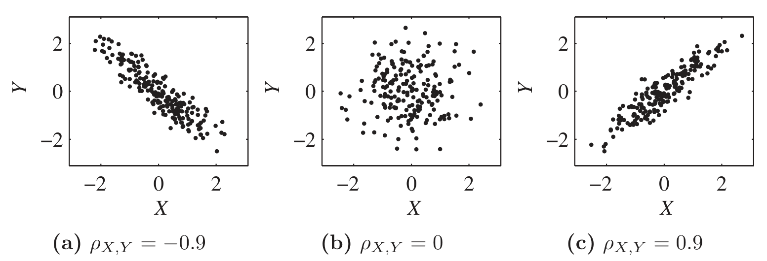
The sign of $\mathrm{Cov}[X,Y]$ reveals the correlation type between $X$ and $Y$:

Correlation	Sign
Positively correlated	$\mathrm{Cov}[X,Y]>0$
Negatively correlated	$\mathrm{Cov}[X,Y]<0$
Uncorrelated	$\mathrm{Cov}[X,Y]=0$

Correlation coefficient

Suppose $X$ and $Y$ are any two random variables on a probability model.

Their correlation coefficient is a rescaled version of covariance that measures the synchronicity of deviations:

$$\rho [X,Y]=\frac{\mathrm{Cov}[X,Y]}{{\sigma }_X{\sigma }_Y}=\mathrm{Cov}[\frac{X}{{\sigma }_X},\frac{Y}{{\sigma }_Y}]$$

The rescaling ensures:

$$-1\le {\rho }_{X,Y}\le +1$$

Covariance depends on the separate variances of $X$ and $Y$ as well as their relationship.

Correlation coefficient, because we have divided out ${\sigma }_X{\sigma }_Y$, depends only on their relationship.

Link to original

10 Illustration

Covariance from PMF chart

Covariance from PMF chart

Suppose the joint PMF of $X$ and $Y$ is given by this chart:

$Y\downarrow X\to$	$1$	$2$
$-1$	0.2	0.2
$0$	0.35	0.1
$1$	0.05	0.1

Find $\mathrm{Cov}[X,Y]$.

Solution

We need $E[X]$ and $E[Y]$ and $E[XY]$.

$$E[X]=1\cdot (0.2+0.35+0.05)+2\cdot (0.2+0.1+0.1)\gg \gg 1.4$$ $$\begin{array}{c}E[Y]=-1\cdot (0.2+0.2)+0\cdot (0.35+0.1)+1\cdot (0.05+0.1)\\ \\ \gg \gg -0.25\end{array}$$ $$E[XY]=-1\cdot (0.2)-2\cdot (0.2)+0+1\cdot (0.05)+2\cdot (0.1)\gg \gg -0.35$$

Therefore:

$$\begin{array}{c}\mathrm{Cov}[X,Y]=E[XY]-E[X]E[Y]\\ \\ \gg \gg -0.35-(1.4)(-0.25)\gg \gg 0\end{array}$$ Link to original

11 Theory

Theory 2

Covariance bilinearity

Given any three random variables $X$, $Y$, and $Z$, we have:

$$\begin{array}{cc}\mathrm{Cov}[X+Y,Z]& =\mathrm{Cov}[X,Z]+\mathrm{Cov}[Y,Z]\\ & \\ \mathrm{Cov}[Z,X+Y]& =\mathrm{Cov}[Z,X]+\mathrm{Cov}[Z,Y]\end{array}$$

Covariance and correlation: shift and scale

Covariance scales with each input, and ignores shifts:

$$\mathrm{Cov}[aX+b,Y]=a\mathrm{Cov}[X,Y]=\mathrm{Cov}[X,aY+b]$$

Whereas shift or scale in correlation only affects the sign:

$$\rho [aX+b,Y]=\mathrm{sign}(a)\rho [X,Y]=\rho [X,aY+b]$$

Extra - Proof of covariance bilinearity

$$\begin{array}{cc}\mathrm{Cov}[X+Y,Z]& \gg \gg E[(X+Y-({\mu }_X+{\mu }_Y))(Z-{\mu }_Z)]\\ & \\ & \gg \gg E[(X-{\mu }_X+Y-{\mu }_Y)(Z-{\mu }_Z)]\\ & \\ & \gg \gg E[(X-{\mu }_X)(Z-{\mu }_Z)]+E[(Y-{\mu }_Y)(Z-{\mu }_Z)]\\ & \\ & \gg \gg \mathrm{Cov}[X,Z]+\mathrm{Cov}[Y,Z]\end{array}$$

Extra - Proof of covariance shift and scale rule

$$\begin{array}{cc}\mathrm{Cov}[aX+b,Y]& \gg \gg E[(aX+b)Y]-E[aX+b]E[Y]\\ & \\ & \gg \gg E[aXY+bY]-aE[X]E[Y]-E[b]E[Y]\\ & \\ & \gg \gg aE[XY]+bE[Y]-aE[X]E[Y]-bE[Y]\\ & \\ & \gg \gg a(E[XY]-E[X]E[Y])\end{array}$$

---

Independence implies zero covariance

Suppose that $X$ and $Y$ are any two random variables on a probability model.

If $X$ and $Y$ are independent, then:

$$\mathrm{Cov}[X,Y]=0$$

Proof:

We know both of these:

$$\begin{array}{ccc}& E[XY]=E[X]E[Y]& \text{(independence)}\\ & & \\ & \mathrm{Cov}[X,Y]=E[XY]-{\mu }_X{\mu }_Y& \text{(shorter form)}\end{array}$$

But $E[XY]=E[X]E[Y]={\mu }_X{\mu }_Y$, so those terms cancel and $\mathrm{Cov}[X,Y]=0$.

Sum rule for variance

Suppose that $X$ and $Y$ are any two random variables on a probability space.

Then:

$$\mathrm{Var}[X+Y]=\mathrm{Var}[X]+\mathrm{Var}[Y]+2\mathrm{Cov}[X,Y]$$

When $X$ and $Y$ are independent:

$$\mathrm{Var}[X+Y]=\mathrm{Var}[X]+\mathrm{Var}[Y]$$

Extra - Proof: Sum rule for variance

$$\begin{array}{cc}\mathrm{Var}[X+Y]& \gg \gg E\left[\right(X+Y-({\mu }_X+{\mu }_Y){)}^2]\\ & \\ & \gg \gg E\left[\right((X-{\mu }_X)+(Y-{\mu }_Y){)}^2]\\ & \\ & \gg \gg E[(X-{\mu }_X{)}^2+(Y-{\mu }_Y{)}^2+2(X-{\mu }_X)(Y-{\mu }_Y)]\\ & \\ & \gg \gg \mathrm{Var}[X]+\mathrm{Var}[Y]+2\mathrm{Cov}[X,Y]\end{array}$$

Extra - Proof that $-1\le \rho \le +1$

(1) Create standardizations:

$$\tilde{X}=\frac{X-{\mu }_X}{{\sigma }_X},\tilde{Y}=\frac{Y-{\mu }_Y}{{\sigma }_Y}$$

Now $\tilde{X}$ and $\tilde{Y}$ satisfy:

$$E[\tilde{X}]=0=E[\tilde{Y}]\text{and}\mathrm{Var}[\tilde{X}]=1=\mathrm{Var}[\tilde{Y}]$$

Observe that $\mathrm{Var}[W]\ge 0$ for any $W$. Variance can’t be negative.

---

(2) Apply the variance sum rule.

Apply to $\tilde{X}$ and $\tilde{Y}$:

$$0\le \mathrm{Var}[\tilde{X}+\tilde{Y}]=\mathrm{Var}[\tilde{X}]+\mathrm{Var}[\tilde{Y}]+2\mathrm{Cov}[\tilde{X},\tilde{Y}]$$

Simplify:

$$\begin{array}{c}\gg \gg 1+1+2\mathrm{Cov}[\tilde{X},\tilde{Y}]\ge 0\\ \\ \gg \gg 1+\mathrm{Cov}[\tilde{X},\tilde{Y}]\ge 0\end{array}$$

Notice effect of standardization:

$$\mathrm{Cov}[\tilde{X},\tilde{Y}]=\rho [X,Y]$$

Therefore $\rho [X,Y]\ge -1$.

---

(3) Modify and reapply variance sum rule.

Change to $\tilde{X}-\tilde{Y}$:

$$0\le \mathrm{Var}[\tilde{X}-\tilde{Y}]=\mathrm{Var}[\tilde{X}]+\mathrm{Var}[-\tilde{Y}]+2\mathrm{Cov}[\tilde{X},-\tilde{Y}]$$

Simplify:

$$\begin{array}{c}\gg \gg 1+1-2\mathrm{Cov}[\tilde{X},\tilde{Y}]\ge 0\\ \\ \gg \gg 1-\mathrm{Cov}[\tilde{X},\tilde{Y}]\ge 0\end{array}$$

Link to original

12 Illustration

Variance of sum of indicators

Variance of sum of indicators

An urn contains 3 red balls and 2 yellow balls.

Suppose 2 balls are drawn without replacement, and $X$ counts the number of red balls drawn.

Find $\mathrm{Var}[X]$.

Solution

Let $X_1$ indicate (one or zero) whether the first ball is red, and $X_2$ indicate whether the second ball is red, so $X=X_1+X_2$.

Then $X_1{X}_2$ indicates whether both drawn balls are red; so it is Bernoulli with success probability $\frac{3}{5}\frac{2}{4}=\frac{3}{10}$. Therefore $E[X_1{X}_2]=\frac{3}{10}$.

We also have $E[X_1]=E[X_2]=\frac{3}{5}$.

The variance sum rule gives:

$$\begin{array}{cc}\mathrm{Var}[X]& =\mathrm{Var}[X_1]+\mathrm{Var}[X_2]+2\mathrm{Cov}[X_1,X_2]\\ & \\ & \gg \gg E[X_1^2]-E{[X_1]}^2+E[X_2^2]-E{[X_2]}^2+2(E[X_1{X}_2]-E[X_1]E[X_2])\\ & \\ & \gg \gg \frac{3}{5}-{\left(\frac{3}{5}\right)}^2+\frac{3}{5}-{\left(\frac{3}{5}\right)}^2+2(\frac{3}{10}-\frac{3}{5}\cdot \frac{3}{5})\gg \gg \frac{9}{25}\end{array}$$Link to original

Exercise - Covariance rules

Covariance rules

Simplify:

$$\mathrm{Cov}[2X+5Y+1,3Y+8W+X+9]$$ Link to original

Exercise - Independent variables are uncorrelated

Dependent but uncorrelated variables

Let $X$ be given with possible values $\{-\mathrm{1,0},+1\}$ and PMF given (uniformly) by $P_X(k)=1/3$ for all three possible $k$. Let $Y=X^2$.

Show that $X$ and $Y$ are dependent but uncorrelated.

Hint: To speed the calculation, notice that $X^3=X$.

Link to original