Repeated trials
01 Theory
Repeated trials
When a single experiment type is repeated many times, and we assume each instance is independent of the others, we say it is a sequence of repeated trials or independent trials.
The probability of any sequence of outcomes is derived using independence together with the probabilities of outcomes of each trial.
A simple type of trial, called a Bernoulli trial, has two possible outcomes, 1 and 0, or success and failure, or
- Write sequences like
for the outcomes of repeated trials of this type. - Independence implies
- Write
and , and because these are all outcomes (exclusive and exhaustive), we have . Then: - This gives a formula for the probability of any sequence of these trials.
A more complex trial may have three outcomes,
- Write sequences like
for the outcomes. - Label
and and . We must have . - Independence implies
- This gives a formula for the probability of any sequence of these trials.
Let
Suppose a coin is biased with
The probability of at least 18 heads would then be:
With three possible outcomes,
02 Illustration
Example - Multinomial: Soft drinks preferred
Reliability
03 Theory
Consider some process schematically with components in series and components in parallel:
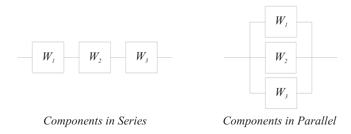
- Each component has a probability of success or failure.
- Event
indicates ‘success’ of that component (same name). - Then
is the probability of succeeding.
Success for a series of components requires success of each member.
- Series components rely on each other.
- Success of the whole is success of part 1 AND success of part 2 AND part 3, etc.
Failure for parallel components requires failure of each member.
- Parallel components represent redundancy.
- Success of the whole is success of part 1 OR success of part 2 OR part 3, etc.
For series components:
For parallel components:
If
- Series components:
- Parallel components:
To analyze a complex diagram of series and parallel components, bundle each:
- pure series set as a single compound component with its own success probability (the product)
- pure parallel set as a single compound component with its own success probability (using the failure formula)
This is like the analysis of resistors and inductors.
04 Illustration
Example - Series, parallel, series
Discrete random variables
05 Theory
Random variable
A random variable (RV)
on a probability space is a function . So
assigns to each outcome a number.
- !!! The word ‘variable’ indicates that the RV outputs numbers.
Random variables can be formed from other random variables using mathematical operations on the output numbers.
Given random variables
Random variables determine events.
- Given
, the event “ ” is equal to the set - That is: the set of outcomes mapped to
by - That is: the event “
took the value ”
Such events have probabilities. We write them like this:
This generalized to events where
The axioms of probability translate into rules for these events.
For example, additivity leads to:
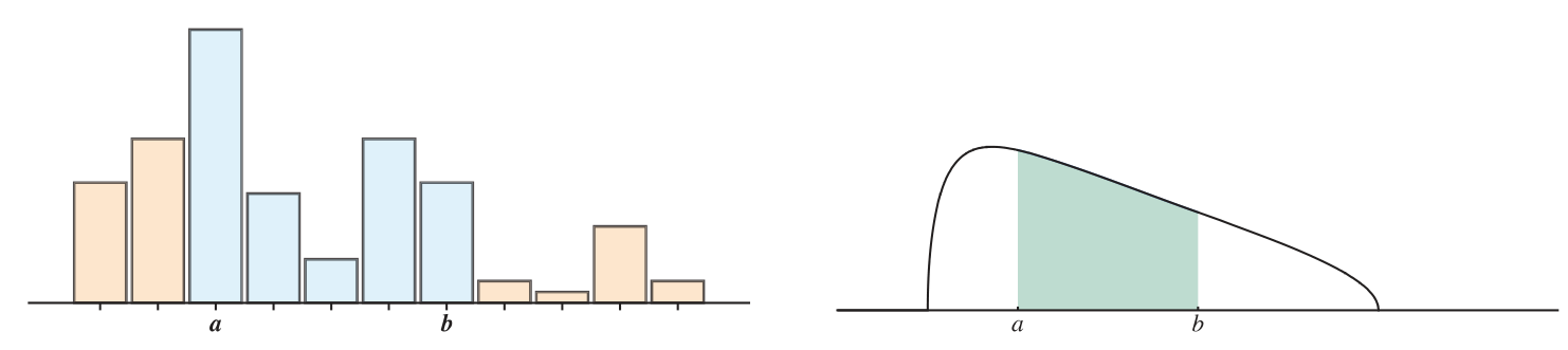
A discrete random variable has probability concentrated at a discrete set of real numbers.
- A ‘discrete set’ means finite or countably infinite.
- The distribution of probability is recorded using a probability mass function (PMF) that assigns probabilities to each of the discrete real numbers.
- Numbers with nonzero probability are called possible values.
PMF
The PMF function for
(a discrete RV) is defined by: for
a possible value.
A continuous random variable has probability spread out over the space of real numbers.
- The distribution of probability is recorded using a probability density function (PDF) which is integrated over intervals to determine probabilities.
The PDF function for
(a CRV) is written for , and probabilities are calculated like this:
For any RV, whether discrete or continuous, the distribution of probability is encoded by a function:
CDF
The cumulative distribution function (CDF) for a random variable
is defined for all by:
Notes:
- Sometimes the relation to
is omitted and one sees just “ .” - Sometimes the CDF is called, simply, “the distribution function” because:
- ! The CDF works equally well for discrete and continuous RVs.
- Not true for PMF (discrete only) or PDF (continuous only).
- There are mixed cases (partly discrete, partly continuous) for which the CDF is essential.
The CDF of a discrete RV is always a stepwise increasing function. At each step up, the jump size matches the PMF value there.
From this graph of 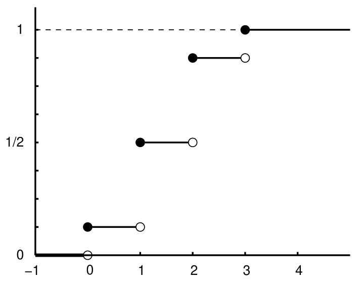
we can infer the PMF values based on the jump sizes:
For a discrete RV, the CDF and the PMF can be calculated from each other using formulas.
PMF from CDF from PMF
Given a PMF
, the CDF is determined by: where is the set of possible values of . Given a CDF
, the PMF is determined by:
06 Illustration
Example - PDF and CDF: Roll 2 dice
Example - Total heads count; binomial expansion of 1
Example - Life insurance payouts