Week 07 notes

Joint distributions

01 Theory

Joint distributions describe the probabilities of events associated with multiple random variables simultaneously.

In this course we consider only two variables at a time, typically called and . It is easy to extend this theory to vectors of random variables.

Joint PMF and joint PDF

Discrete joint PMF:

Continuous joint PDF:

Probabilities of events: Discrete case If is a set of points in the plane, then an event is formed by the set of all outcomes mapped by and to points in :

The probabilities of such events can be measured using the joint PMF:

Probabilities of events: Continuous case Let be the rectangular region defined by such that and . Then: For more general regions :

---

The existence of a variable does not change the theory for a variable considered by itself.

However, it is possible to relate the theory for to the theory for , in various ways.

The simplest relationship is the marginal distribution for , which is merely the distribution of itself, considered as a single random variable, but in a context where it is derived from the joint distribution for .

Marginal PMF, marginal PDF

Marginal distributions are obtained from joint distributions by summing the probabilities over all possibilities of the other variable.

Discrete marginal PMF:

Continuous marginal PMF:

---

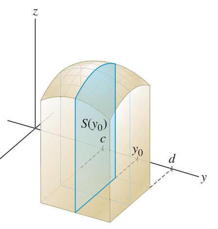
Infinitesimal method

Suppose has density that is continuous at . Then for small :

Suppose and have joint density that is continuous at . Then for small :

Joint densities depend on coordinates

The density in these integration formulas depends on the way and act as Cartesian coordinates and determine differential areas as little rectangles.

To find a density in polar coordinates, for example, it is not enough to solve for and and plug into . We must consider the differential area vs. . We find that . So we will add a factor of . See an example below for details.

Joint densities may not exist

It is not always possible to form a joint PDF from any two continuous RVs and .

For example, if , then cannot have a joint PDF, since but the integral over the region will always be 0. (The area of a line is zero.)

02 Illustration

Example - Smaller and bigger rolls

Exercise - Reading a PMF table

Exercise - Coin flipping

Example - Marginal and event probability from joint density

Exercise - Marginals from joint density

Exercise - Event probability from joint density

03 Theory

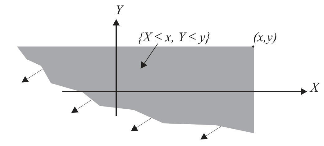
Joint CDF

The joint CDF of and is defined by:

We can relate the joint CDF to the joint PDF using integration:

Conversely, if and have a continuous joint PDF that is also differentiable, we can obtain the PDF from the CDF using partial derivatives:

---

There is also a marginal CDF that is computed using a limit:

This could also be written, somewhat abusing notation, as .

04 Illustration

Exercise - Properties of joint CDFs

(a) Show with a drawing that if both and , we know:

(b) Explain why:

(c) Explain why:

Independent random variables

05 Theory

Independent random variables

Random variables are independent when they satisfy the product rule for all valid subsets :

Since , this definition is equivalent to independence of all events constructible using the variables and .

For discrete random variables, it is enough to check independence for simple events of type and for and any possible values of and .

---

The independence criterion for random variables can be cast entirely in terms of their distributions and written using the PMFs or PDFs.

Independence using PMF and PDF

Discrete case:

Continuous case:

Independence via joint CDF

Random variables and are independent when their CDFs obey the product rule:

06 Illustration

Example - Meeting in the park

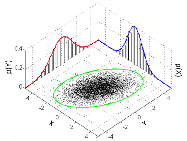
Example - Uniform disk: Cartesian vs. polar