Functions on two random variables
01 Theory
PMF of any function of two variables
Suppose
and are discrete RVs. The PMF of
:
CDF of continuous function of two variables
Suppose
and are continuous RVs, and is a continuous function. The CDF of
:
One can then compute the PDF of
02 Illustration
Example - PDF of a quotient
Exercise - PMF of
from chart
Example - Max and Min from joint PDF
Sums of random variables
03 Theory
The special case where
THEOREM: Continuous PDF of a sum
Suppose
is the joint PDF for continuous RVs and . Then the PDF
of is given by the formula: When
and are independent, so , the formula turns into the convolution of and :
- ! There is no particular reason to choose the
-slot for . - Equally valid to write:
- Equally valid to write:
Extra - Derivation of continuous PDF of a sum
The joint CDF of
is given by: From this we can find
by taking the derivative: In order to calculate this derivative, we change variables by setting
and . The Jacobian is 1, so becomes , and we have:
04 Illustration
Example - Sum of parabolic random variables
THEOREM: Discrete PMF of a sum
Suppose
is the joint PMF for discrete RVs and .F Assume that the possible value pairs are
with (integers only). Then the PMF of
is given by the formula:
PMF of
for discrete variables
05 Theory
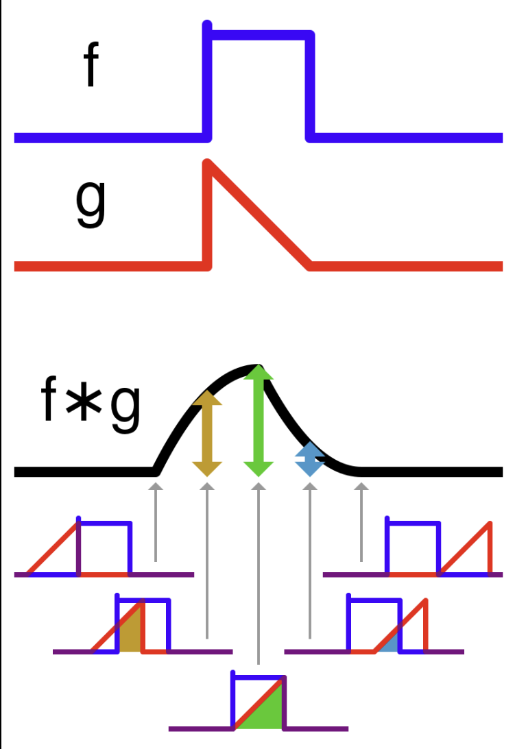
Convolution
The convolution of two continuous functions
and is defined by:
For more example calculations, look at 9.6.1 and 9.6.2 at this page.
Applications of convolution
- Convolutional neural networks (machine learning theory: translation invariant NN, low pre-processing)
- Image processing: edge detection, blurring
- Signal processing: smoothing and interpolation estimation
- Electronics: linear translation-invariant (LTI) system response: convolution with impulse function
Extra - Convolution
Geometric meaning of convolution Convolution does not have a neat and precise geometric meaning, but it does have an imprecise intuitive sense.
The product of two quantities tends to be large when both quantities are large; when one of them is small or zero, the product will be small or zero. This behavior is different from the behavior of a sum, where one summand being large is sufficient for the sum to be large. A large summand overrides a small co-summand, whereas a large factor is scaled down by a small cofactor.
The upshot is that a convolution will be large when two functions have similar overall shape. (Caveat: one function must be flipped in a vertical mirror before the overlay is considered.) The argument value where the convolution is largest will correspond to the horizontal offset needed to get the closest overlay of the functions.
Algebraic properties of convolution
The last of these is not the typical Leibniz rule for derivatives of products!
All of these properties can be checked by simple calculations with iterated integrals.
Convolution in more variables Given
, their convolution at is defined by integrating the shifted products over the whole domain:
06 Illustration
Exercise - Convolution practice
07 Theory
Some pairs of density functions have convolutions that can be described neatly in terms of the densities of known distributions, and sometimes this relationship has its own interpretation in the applied context of a probability model.
Bernoulli plus Binomial
Suppose
for are independent Bernoulli variables. Define
, and notice that . Then
where . In other words: adding a Bernoulli to a Binomial creates a bigger Binomial.
Extra - Proof of Bernoulli sum rule
For the PMF of
, we have for , and for other . For the PMF of
we have for and for other . We seek the discrete convolution
. The factor
in the convolution is nonzero only when or . So we have: This is the PMF of
, so we are done.
Binomial sum rule
Suppose
and are independent RVs with the given binomial distributions (same , different numbers of trials). Then
.
Extra - Proof of binomial sum rule
Of course,
measures the number of successes in independent trials, each with success probability .
08 Illustration
Exercise - Vandermonde’s identity from the binomial sum rule
09 Theory
Recall that a Poisson variable counts ‘arrivals’ in a fixed time window. It applies to events like phone calls per hour or Uranium decays per second. Each interval is independent of the others, and the rate of occurrences is proportional to the size of the interval.
An implication of this meaning of the Poisson variable is a sum rule. If you divide a Poisson interval into subintervals, the distribution corresponding to each subinterval should still be Poisson, and the distribution of arrivals in each subinterval should add up to give the distribution of arrivals for the total interval.
Poisson sum rule
Suppose
and and and are independent. Then
.
Extra - Proof of Poisson sum rule
Write
and . Then:
Recall that in a Bernoulli process:
- An RV measuring the discrete wait time until one success has a geometric distribution.
- An RV measuring discrete wait time until
success has a Pascal distribution.
Since the wait times between successes are independent, we expect that the sum of geometric distributions is a Pascal distribution. This is true!
Pascal Sum Rule
Specify a given Bernoulli process with success probability
. Suppose that:
and are independent Then
.
Geom plus Geom is Pascal
Recall that
. So we could say: And:
The Pascal Sum Rule can be justified in two ways:
- (1) by directly computing the discrete convolution of two Pascal variables
- (2) by observing that the sum
counts the trials until exactly successes - Waiting for
successes and then waiting for successes is the same as waiting for successes
- Waiting for
Recall that in a Poisson process:
- An RV measuring continuous wait time until one arrival has an exponential distribution.
- An RV measuring continuous wait time until
arrival has an Erlang distribution.
Since the wait times between arrivals are independent, we expect that the sum of exponential distributions is an Erlang distribution. This is true!
Erlang sum rule
Specify a given Bernoulli process with success probability
. Suppose that:
and are independent Then
.
Exp plus Exp is Erlang
Recall that
. So we could say: And:
10 Illustration
Example - Exp plus Exp equals Erlang
Exercise - Erlang induction step
By repeated iteration of the above formula, starting with
This fully explains the formula for the Erlang PDF.
11 Theory
Normal sum rule
Suppose we know:
and are independent Then:
Recall that
This fact, combined with the sum rule, implies that
12 Illustration
Combining normals