Statistical testing cont’d
01 Theory - Binary testing, MAP and ML
Binary hypothesis test
Ingredients of a binary hypothesis test:
- Complementary hypotheses
and
- Maybe also know the prior probabilities
and - Goal: determine which case we are in,
or - Decision rule made of complementary events
and
is likely given , while is likely given - Decision rule: outcome
, accept ; outcome , accept - Usually:
written in terms of decision statistic using a design - We cover three designs:
- MAP and ML (minimize ‘error probability’)
- MC (minimizes ‘error cost’)
- Designs use
and (or , ) to construct and
MAP design
Suppose we know:
- Both prior probabilities
and - Both conditional distributions
and (or and ) The maximum a posteriori probability (MAP) design for a decision statistic
:
Discrete case:
Continuous case:
Then
. The MAP design minimizes the total probability of error.
ML design
Suppose we know only:
- Both conditional distributions
The maximum likelihood (ML) design for
:
ML is a simplified version of MAP.
(Set and to .)
The probability of a false alarm, a Type I error, is called
The probability of a miss, a Type II error, is called
Total probability of error:
False alarm
false alarm Suppose
sets off a smoke alarm, and is ‘no fire’ and is ‘yes fire’. Then
is the odds that we get an alarm assuming there is no fire. This is not the odds of experiencing a false alarm (no context). That would be
. This is not the odds of a given alarm being a false one. That would be
.
02 Illustration
Example - ML test: Smoke detector
Example - MAP test: Smoke detector
03 Theory - MAP criterion proof
Explanation of MAP criterion - discrete case
First, we show that the MAP design selects for
all those which render more likely than . Observe this Calculation:
Now, take the condition for
, and cross-multiply:
Divide both sides by
and apply the above Calculation in reverse:
This is what we sought to prove.
Next, we verify that the MAP design minimizes the total probability of error.
The total probability of error is:
Expand this with summation notation (assuming the discrete case):
Now, how do we choose the set
(and thus ) in such a way that this sum is minimized? Since all terms are positive, and any
may be placed in or in freely and independently of all other choices, the total sum is minimized when we minimize the impact of placing each . So, for each
, we place it in if:
That is equivalent to the MAP condition.
04 Theory - MC design
- Write
for cost of false alarm, i.e. cost when is true but decided . - Probability of incurring cost
is .
- Probability of incurring cost
- Write
for cost of miss, i.e. cost when is true but decided . - Probability of incurring cost
is .
- Probability of incurring cost
Expected value of cost incurred
MC design
Suppose we know:
- Both prior probabilities
and - Both conditional distributions
and (or and ) The minimum cost (MC) design for a decision statistic
:
Discrete case:
Continuous case:
Then
. The MC design minimizes the expected value of the cost of error.
MC minimizes expected cost
Inside the argument that MAP minimizes total probability of error, we have this summation:
The expected value of the cost has a similar summation:
Following the same reasoning, we see that the cost is minimized if each
is placed into precisely when the MC design condition is satisfied, and otherwise it is placed into .
05 Illustration
Example - MC Test: Smoke detector
Mean square error
06 Theory - Minimum mean square error
Suppose our problem is to estimate or guess or predict the value of a random variable
There is no single best answer to this question. The best answer is a function of additional factors in the problem context.
One method is to pick a value where the PMF or PDF of
Another method is to pick the expected value
For the normal distribution, or any symmetrical distribution, these are the same value. For most distributions they are not the same value.
Mean square error
Given an estimate
for a random variable , the mean square error (MSE) of is:
The MSE quantifies the typical (square of the) error, meaning the difference between the true value
Other error estimates are reasonable and useful in niche contexts. For example,
In problem contexts where large errors are more costly than small errors (many real problems), the most likely value of
It turns out the expected value
Minimal mean square error
Given a random variable
, its expectation provides the estimate with minimal mean square error. The MSE error itself of
:
Proof that
gives minimal MSE Expand the MSE error:
Minimize this parabola. Differentiate:
Find zeros:
When the estimate
In the presence of additional information, namely that event
The MSE estimate can also be conditioned on another variable, say
Minimal MSE of
given The minimal MSE estimate of
given another variable :
The error of this estimate is
, which equals .
Notice that the minimal MSE of
This variable is a derived variable of
The variable
07 Illustration
Example - Minimal MSE estimate given PMF, given fixed event
Exercise - Minimal MSE estimate from joint PDF
08 Theory - Line of minimal MSE
Linear approximation is very common in applied math.
One could consider the linearization of
Instead, one can minimize the MSE over all possible linear functions of
Line of minimal MSE
Let
be the line . Let . The mean square error (MSE) of
is:
The linear estimator is the line
with minimal MSE, and it is:
The minimal error value
is:
The variable of minimal error,
, is uncorrelated with .
Slope and
Notice:
Thus,
is the slope of the minimal MSE line for standardized variables and .
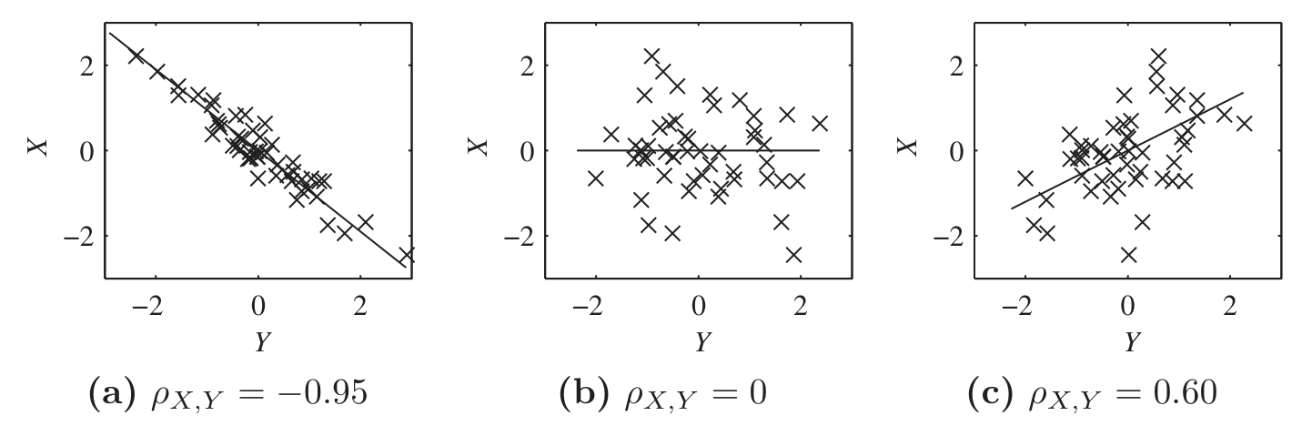
In each graph,
The line of minimal MSE is the “best fit” line,
09 Illustration
Example - Estimating on a variable interval
Exercise - Line of minimal MSE given joint PDF