TDA in pictures
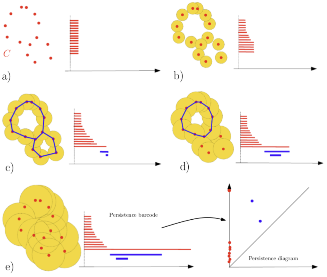
Detecting topological features with a filtration:
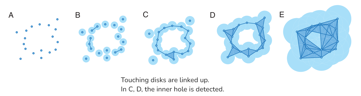
“Barcodes” of persistence homology:
Topological spaces: basic notions
01 Theory - Spaces, subspaces, connectedness
Topological space
A topological space is a set (the ‘space’) together with a topology structure.
A topology structure is a determination of open subsets of .
Formally: open sets are collected together in a set of sets , the topology.
Open sets (in ) must satisfy axioms:
- and are open
- All unions of opens are open
- Finite intersections of opens are open
A set is called closed when is open.
Although these axioms for open sets seem rather obscure, a long history (leading up to and in consequence of the axioms) has shown that the concept of open set they determine accurately formalizes our intuitions about spatial connectedness, and the aspect of proximity that underwrites connectedness.
Many geometric sets have natural topology structures:
Some notes:
- The trivial topology has only the minimum of open sets, and .
- The discrete topology has the maximum of open sets, . (All subsets are open.)
- Sometimes a set is simultaneously closed and open, thus ‘clopen’. E.g. and are always clopen.
Subspace topology
For any subset , there is a subspace topology structure on .
The open sets of are the intersections where is open in .
Beware that open sets in a subspace topology might not be open in itself.
Connectedness
A topological space is connected when it is impossible to decompose it as a disjoint union of opens:
02 Illustration
Simple topology - connectedness
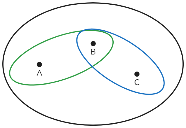
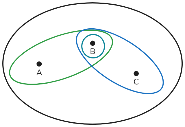
Three points: , with two (nontrivial) open sets. This is not a topology because the intersection is not open:
This is a topology, and it is connected:
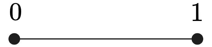
Continuum - real number interval
The standard topology structure for real numbers is generated by open intervals .
(“Generated”: it is the smallest topology structure containing all such intervals.)
In D, the open sets are generated by open boxes or (equivalently) open balls .
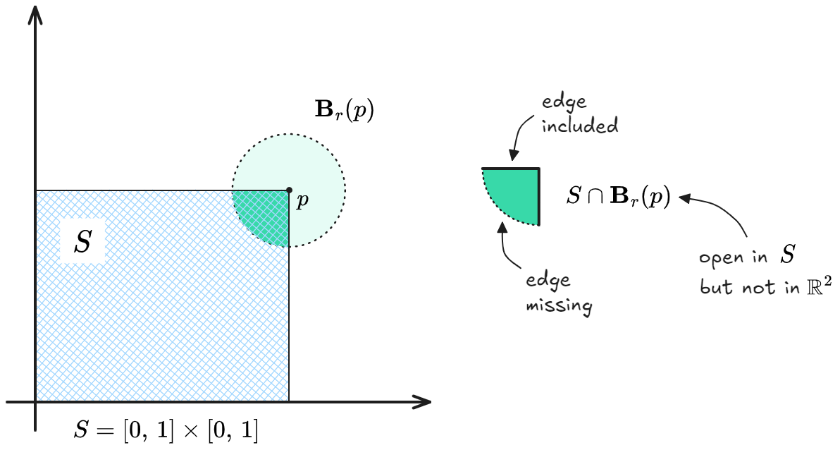
Open in but not in
Consider the subspace equipped with the subspace topology inherited from the topology structure on :
An open set in may be given as the intersection with a ball in , but this set is not open in because the top and right edges would be included. No open ball can be found around a point in this edge and contained in .
03 Theory - Metric, open balls, continuity
Metric space
A metric space is a set (the ‘space’) together with a metric structure.
A metric structure is a determination of distance between points in the set.
Formally: distance is measured by a function satisfying: Triangle inequality:
and more basic axioms:
- for all
In the distance function is, of course, .
Using any distance function, we can define open balls:
Then we can generate a topology on from these open balls. We are, in effect, using the topology of in the codomain of to induce a topology back on the space .
Metric space topology
Any metric space has a natural metric space topology structure.
The open sets are generated by open balls . That is, open sets are all unions of open balls:
Every structure of metric space automatically has a natural structure of topological space due to the above definition.
A topology structure formalizes only the notion of connectedness, or one might say “touching vs. separated”, while a metric structure adds a quantitative measure of distance. As such it implies notions like “double the distance” or “ the distance.” But a metric structure does imply at least a topology structure, because any points that are separated by some distance are in fact separated.
Topological structures that do not come from metric structures can also be useful and interesting. (E.g. in algebraic geometry.) But the notion of “touching” that they express is rather abstracted from the geometrical one we are accustomed to.
“All unions of open balls”
The collection “all unions of open balls” satisfies the axioms of a topology. The first two axioms clearly hold. To check the third axiom, one would have to formalize the concept of ‘generates’, which is applicable to the concept of ‘subbase’. The essential verification is that for any point inside a finite intersection of open balls, there is another open ball around that point which is contained in the intersection. The triangle axiom is needed to confirm this.
LEMMA: open subsets via open balls
In any metric space , a subset is open if and only if:
In words: is open IFF any in has some open ball around it which is contained in .
This lemma provides a functional characterization of open sets in a metric space.
Proof of LEMMA
Assume the Lemma condition holds; try to prove is open.
- For each , write for some open ball over contained in . Then , and is a union of open sets, thus open.
Now assume is open; try to prove the condition holds.
- is necessarily the union of some open balls. (Definition of topology structure given a metric.)
- Select any . By 1., this is in some open ball :
- Find a ball centered at which is inside , thus inside .
- Set
- Definition of ball and implies
- Set
- Triangle Inequality: Every satisfies
- Therefore
Continuous functions
A function between topological spaces is continuous when:
This definition implies that a connected subset cannot be mapped to a disconnected subset by a continuous . Given any disjoint union of opens that ‘disconnects’ the image of , the definition implies that and are disjoint opens covering and disconnecting it. The fact that the definition of continuity appears to go “the wrong way” (implication from codomain to domain ) is related to the logical negation inside “no possible disjoint union of opens” in the definition of connectedness.
For example, the graph of a function with a jump discontinuity:
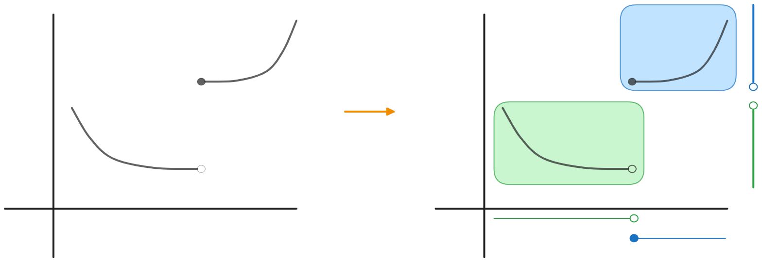
The disconnected image of can be separated by open sets in the codomain (vertical axis). The domain is not separated by the preimages – the function is not continuous.
An equivalent definition of continuity can be cast in terms of the metric structure, if the topology comes from a metric:
Continuity and distance
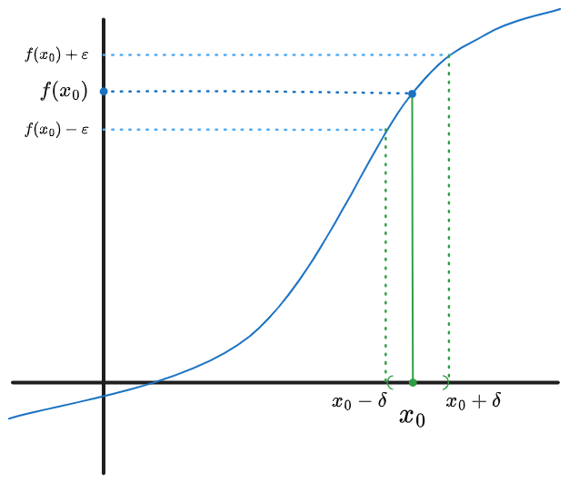
A map of metric spaces is continuous at when:
For all , there exists such that:
Then itself is continuous if it is continuous at every point .
04 Illustration
In Calc I we learn that is continuous at when:
Or, in terms of set containment:
Let us compare this to the definition in terms of open sets:
Open-set continuity agrees with - continuity
Assume that is continuous according to the topological definition.
- Select any . Let be given.
- The interval is open.
- By the topological definition of continuity, the preimage is open. It contains .
- By the Lemma for metric space continuity, find an open ball around inside .
- This ball is an interval .
- All elements of this interval are mapped into , confirming the - condition.
Assume that is continuous according to the - definition.
- Select any open set. We must show is open.
- Select any . Define .
- Then , and so for some by metric space continuity.
- This is an interval:
- By the - definition of continuity, produce some so that:
- Therefore, whenever , we know .
- So is open (by definition), is contained in , and contains , confirming the topological continuity condition.
05 Theory - Compactness, homeomorphism, continuity, homotopy
Compactness
A topological space is compact when every open cover has a finite subcover.
The entire real line is not compact because the open cover has no finite subset which also covers .
The closed interval is compact.
- Let be any open cover of .
- Define :
- Let be the supremum of .
- We show .
- Suppose and seek a contradiction.
- Take some open set in containing , and an open ball around and contained in .
- Move leftwards to . There is a finite cover of from .
- Add to this cover, and get a finite cover of .
- This contradicts the supremum property of . So we know .
- Take some open set in containing , and an open ball .
- There is a finite cover of because .
- Add to this cover to get a finite cover of . QED
Homeomorphism
A homeomorphism is a map between topological spaces, , satisfying:
- is bijective
- is continuous
- is continuous
PROP: ‘Homeomorphism’ simplifies for compact metric spaces
If is a continuous bijection between metric spaces, and and are both compact, then is necessarily a homeomorphism.
Homotopy
A homotopy is a morphism between continuous maps.
Given continuous maps, a homotopy is a continuous function:
We say and are homotopic if any homotopy exists between them.
A homotopy is a continuous deformation of into . Define to view it this way.
For example, suppose we have two maps :
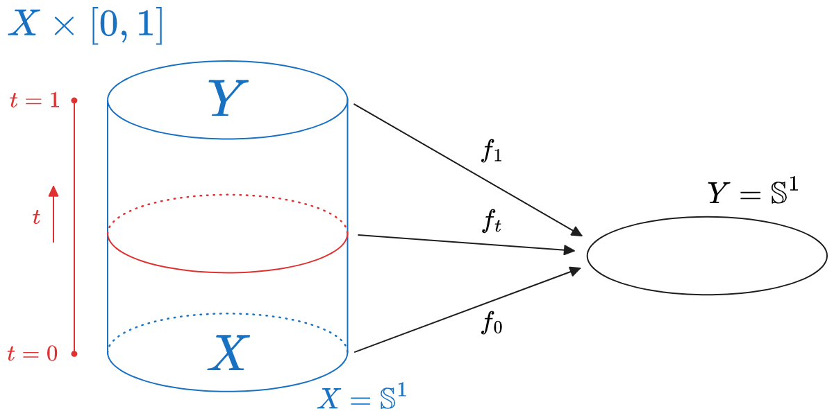
The “winding number” is preserved by , meaning that each has the same winding number.
Topological spaces: further notions
06 Theory - Quotients, gluing
Quotient topology
For any partition of of into cells , , there is a quotient topology structure on the set of cells .
The open sets of are the collections of cells whose unions are open in .
A quotient space is therefore given by ‘collapsing’ some sets of points in into single objects , and the open sets come from open sets in that are compatible with the partition, meaning they do not cross partition boundaries, or that they contain only whole cells.
There are many equivalent formulations of this notion, and these two are most common:
- Using an equivalence relation on , whereby the equivalence classes determine cells of the partition. Then the quotient space is written .
- Recall that partitions and equivalence relations are interchangeable notions.
- Using a surjective function , whereby the preimage fibers determine cells of the partition. Then has the quotient topology when open sets are given by where is open in .
Gluing
Two spaces and can be glued along specified subsets and using a bijection by defining the quotient topology where identifies with .
07 Illustration
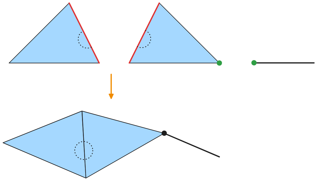
Gluing shapes
- Glue a pair of triangles along an edge.
- Glue a line segment to a triangle, endpoint to vertex.
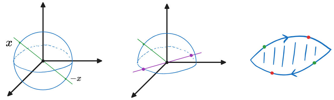
Real projective space
Consider the unit sphere . Antipodal points of are those determining a straight line passing through the origin.
Define as the quotient where equivalence classes of are the pairs of antipodal points.
Define similarly by gluing together antipodal points in .
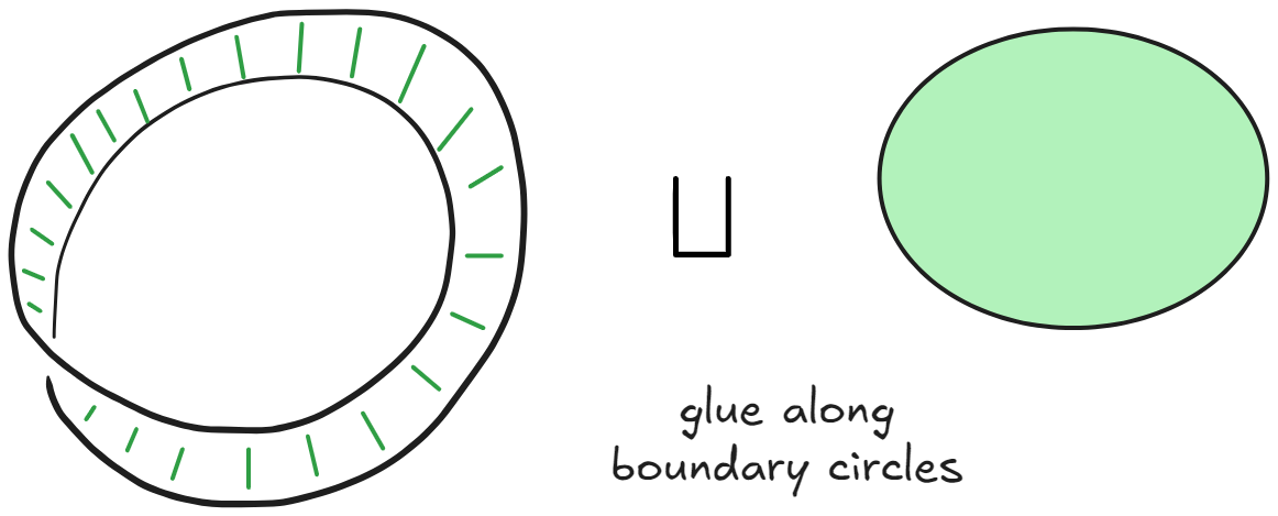
We can also describe using a disk with antipodally glued boundary:
This surface is also derivable by gluing a disk to a Mobius band:
08 Theory - Embedding, limit points, closure, boundary
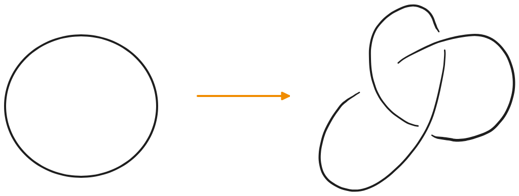
Embedding
An embedding is a continuous injective map that induces a homeomorphism .
It is important to emphasize that should have the subspace topology inherited from .
For example, a knot in is an embedding .
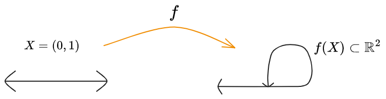
Exercise - Touching upon
An open interval is mapped into by such that one end has a limit point on the image of the middle.
The map is continuous and bijective. Show that is not continuous.
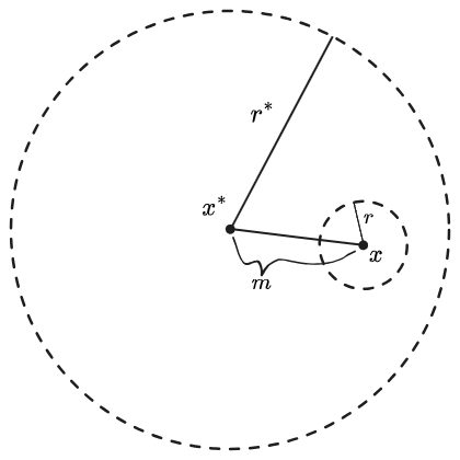
Limit points
Given a subspace , a point is a limit point of when every open set around touches somewhere besides .
Notes:
- Limit points are sometimes called accumulation points.
- The limit point might be outside !
- In a metric space, this can be reformulated: is a limit point of when there is some sequence such that as . This is written .
- In other words, is “approached” from inside .
Interior and exterior
The interior of a set is the set of points with an open neighborhood contained in .
The exterior of a set is the interior of the complement of .
Closure of a set
The closure of a set is the union of with all limit points of .
- Equivalently: the closure is the complement of the union of all open sets in that don’t touch .
- Equivalently: the closure is the intersection of all closed sets containing .
Boundary of a set
The boundary of a set is the set of points in both and .
- Equivalently: the boundary is the set of points for which every open neighborhood touches both the interior and the exterior of .
- Boundary points are not always in !
Simplicial complexes
A simplicial complex is an assembly of simplices, which generalize triangles and tetrahedra. Simplices provide “building block” objects in each dimension that may be glued together to form a complex.
Simplices provide a combinatorial method of representing a large class of topological spaces, since the ‘assembly data’ encoding the gluing of simplices into a complex is combinatorial in nature.
Simplicial homology is a homology theory (topological invariant) that is naturally defined in terms of a given simplicial complex. It is easy to find this homology for a space when a representation as simplicial complex is known.
Simplicial homology is isomorphic to other homology theories.
- Singular homology: abstract ‘naturality’; proving invariance is easier
- Simplicial homology: combinatorial; build complexes by gluing faces ‘directly’; stricter gluing rules
- Delta homology: combinatorial, like simplicial; more relaxed gluing rules
- CW homology: combinatorial, like simplicial but gluing cells (balls) not simplices; build CW complexes inductively; very relaxed gluing rules
For smooth manifolds, we also have:
- De Rham cohomology: uses differential forms “closed but not exact”
09 Theory - Simplices and complexes
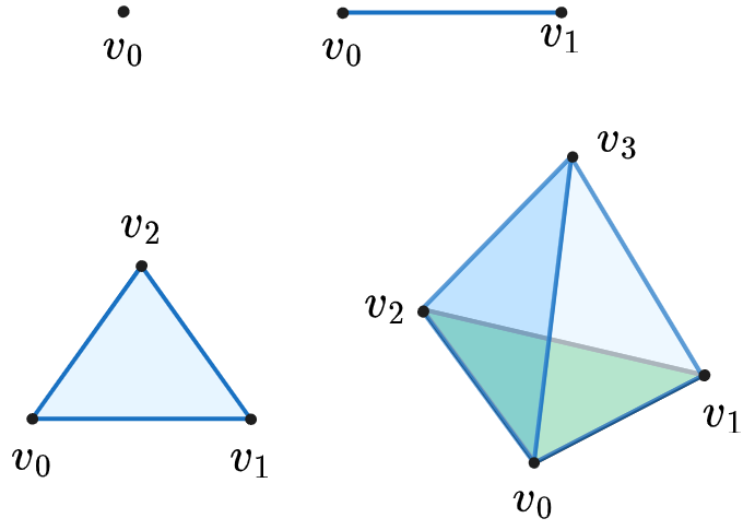
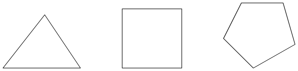
:
- A -simplex is a point (a vertex).
:
- A -simplex is a line segment.
:
- A -simplex is a triangle (interior included).
:
- A -simplex is a tetrahedron.
Geometric simplex
Vertices: , required to be affinely independent.
Geometric simplex:
- Thus is the “convex hull” of . In other words: all weighted averages of the vertices.
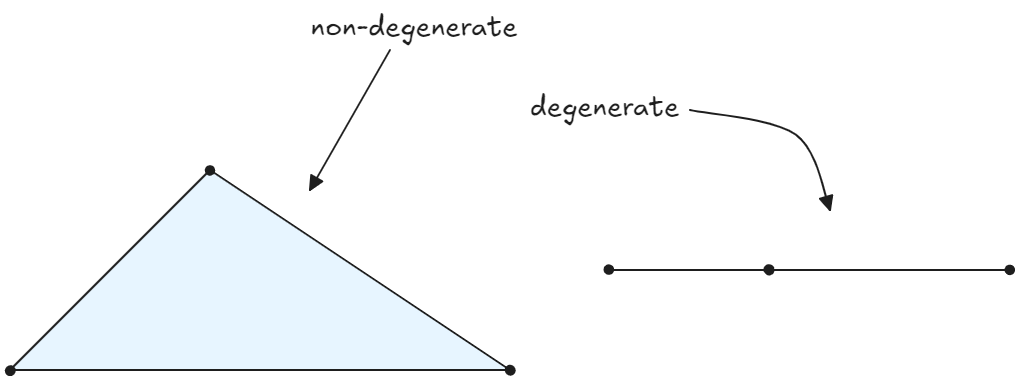
- Affinely independent means: do not lie in any hyperplane (dimension ) of ; equivalently that are linearly independent, or that they generate a vector space of dimension .
- A simplex failing this criterion is called degenerate.
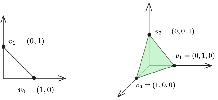
- Standard -simplex : vertices are the unit vectors in .
For example, with the standard simplex is:
This defines the line segment from to .
Similarly, with we find that is parametrized by .
A simplicial complex can be characterized in several ways:
- Combinatorially
- Geometrically
- Topologically
Simplicial complex - Combinatorial
A combinatorial simplical complex with a set of ‘vertices’ is a collection of subsets of , called ‘simplices’, satisfying:
- All faces included: If , then all faces of are in . (And thus faces of faces, all the way down to vertices.)
- Touching only at a face: If , and , then is a face of and a face of .
For , the faces of are the subsets of lacking a single vertex of .
A simplicial complex has a topology. This is given by gluing the disjoint union of constituent simplices along the faces that intersect. (The quotient topology.)
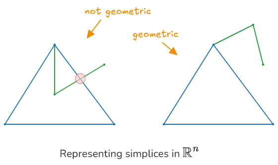
If the simplicial complex is given a geometric representation in , then the glued/quotient topology should match the one inherited by the complex as a subspace of .
10 Illustration
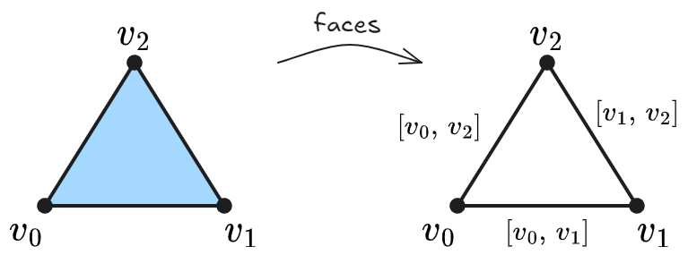
For example, given a simplex , the faces are and and :
A simplicial complex with D subcomplex and D subcomplex and D subcomplex .
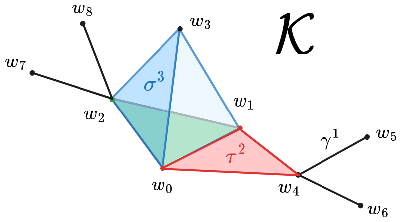
Simplices of dimension are called vertices, simplices of dimension are called edges, and simplices of dimension in an D complex are called faces.
The simplices of top dimension are sometimes called facets (i.e. the biggest ones are called ‘little faces’).
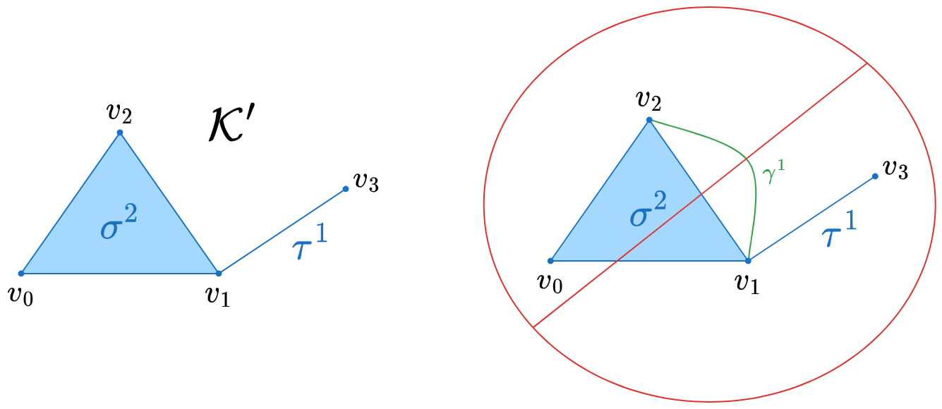
The intersection of two sub-simplices is allowed to be a single face, not two faces (vertices, in this case):
Torus as simplicial complex
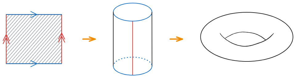
It is easy to create a torus by gluing the edges of a square:
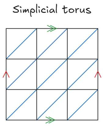
But it is not this easy to represent a torus as a simplicial complex. Initial attempts fail:
One can do it with a little more work and complexity:
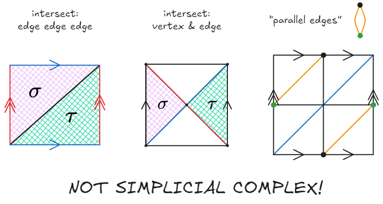
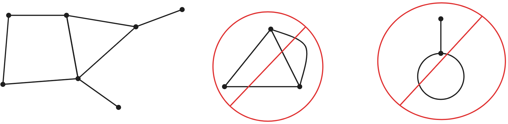
Every finite simple undirected graph is a simplex.
- No “parallel edges”
- No “one-loops”
In a geometric representation of a simplicial complex, edges should not cross, etc.
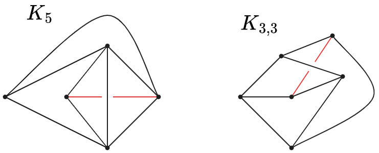
Kuratawki: Graph planarity
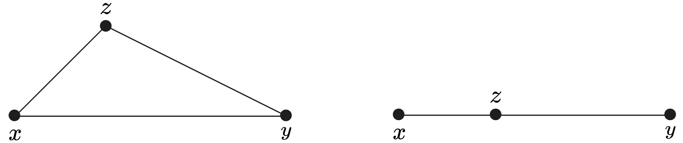
The graph planarity theorem of Kuratowski says that a graph is planar (can be drawn in without self intersection) if and only if it does not contain a copy of or :
11 Theory - Subdivision and triangulation
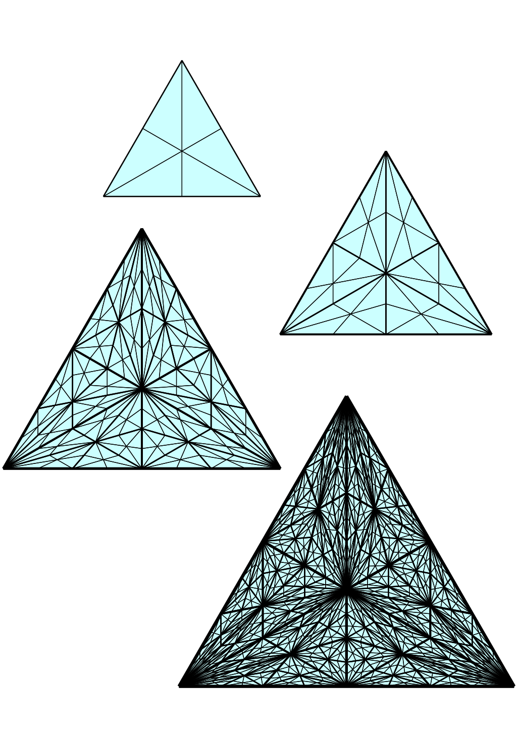
A single topological space (up to homeomorphism) can be represented in many different ways as a simplicial complex:
One can perform “barycentric subdivision” upon a given simplicial complex. This produces a simplicial complex that is homeomorphic to the original one, but the edges are shorter and areas of faces smaller.
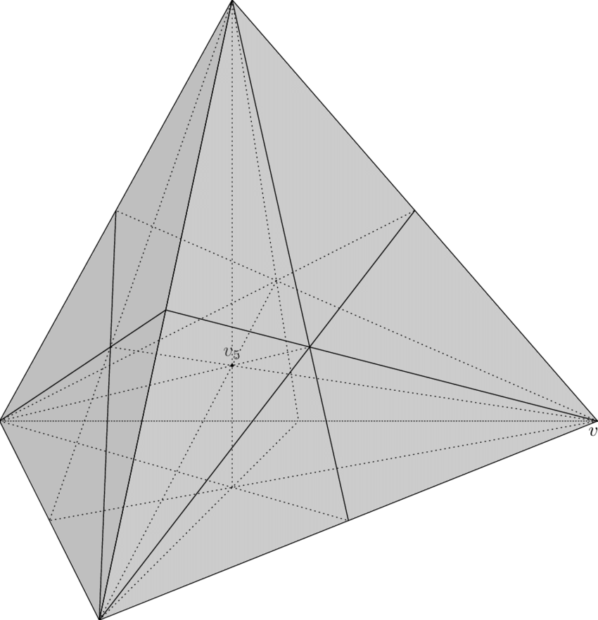
A triangulation is a simplicial complex that is homeomorphic to a given smooth manifold. A triangulated manifold is a simplicial complex together with a homeomorphism to a given smooth manifold.
For example, the tetrahedron obtained by gluing four copies of the standard -simplex is homeomorphic to and is therefore a triangulation of .
Triangulations of spheres
For , all possible triangulation types have been found by Tutte.
For , there is not a known enumeration of triangulation types.
Simplicial homology
Simplicial homology can be defined with “coefficients in ” or with “coefficients in ” (or another ring). Using gives abelian groups, while using gives vector spaces. Vector spaces are nicer to work with, but some information is lost. (Generators of finite order are lost, for example.)
12 Theory - Boundaries, chain complexes
Fix a simplicial complex which is -dimensional. (Highest dimension of a simplex in is .)
Chain groups
For each , , define the chain group :
In other words:
An element of the -chain group, written generically as , is called a -chain.
- Sometimes is dropped and we write just when the complex is clear from context.
By allowing combinations of simplices with coefficients, we can define a boundary operator with alternating signs. This alternation leads to cancellation when boundaries of boundaries are taken. The cancellation in turn enables the definition of homology, which is generated by cycles of simplices that are not boundaries.
Boundary operator
The boundary operator maps simplices to their boundaries. It is defined on simplices and extended linearly to chains:
Examples:
- A -simplex:
- A -simplex:
Orientation and vertex ordering
A simplex was initially defined as the convex closure of a set of points. The points were not ordered! The simplex was not ordered!
The boundary map was defined for an ordered list of points (“ omitted”). These definitions are not compatible!
Let us upgrade both definitions to employ oriented sets of points.
Hereafter, the notation will indicate an ordered list of vertex points up to the equivalence relation that identifies lists which are related by an even permutation.
For example: , but: .
- With this convention, the boundary map is well-defined.
- Notice that the orientation of the vertex list determines the sign of its boundary:
- Therefore: one may interpret the sign of a coefficient in as indicating the orientation of the simplex it is attached to.
- Thus the boundary of a 2-simplex (filled triangle) is an oriented path around the triangle:
LEMMA: Boundary of boundary is empty
For all , we have:
Proof of LEMMA
Apply the double boundary to a generator of :
The second summation duplicates the terms of the first summation, but has one fewer power of , so the whole sum vanishes. Both summations cover all -simplices omitting some two vertices.
Using this fact we construct the chain complex of group homomorphisms:
Chain complex
Given a simplicial complex of maximal dimension , we define the chain complex of as the sequence of morphisms:
This sequence is a complex because the Lemma ensures that
The image and kernel groups have names:
- — called the boundary chains
- — called the cycles
Homology
The homology of is defined as the quotient group of cycles modulo boundary chains:
Notice that in appears in the numerator. So is generated by chains of -simplices.
13 Illustration
Homology of a triangle
Consider the 1D simplicial complex consisting of a triangle:
The chain complex is:
The group is generated by the 1-simplices:
The group is generated by the 0-simplices:
The boundary operator:
The kernel of is freely generated by . The image of is isomorphic to via the map determined by .
So we have and . Higher homology groups vanish.

Homology counts holes by dimension
Consider the space , the wedge sum of three copies of and one copy of obtained by gluing all spaces at a single point:
The homology of this space is:

Homology independent loops in a graph
The “nullity” of a connected graph is the number of independent cycles in the graph. If for a graph considered as a simplicial complex, then is the nullity.
So for the following graph:
