TDA Notes - Unit 02

Delta, Nerve, Čech complexes

01 Theory - Delta complexes

The $\mathrm{\Delta }$-complex structure is a generalization of simplicial complex structure. Instead of gluing simplices from the same ${ℝ}^{n+1}$ by causing them to intersect at faces, one glues simplices from disjoint copies of ${ℝ}^{n+1}$ using a formal quotient topology construction.

This technique allows many common spaces to be represented using fewer simplices. For example, a circle may be given as a $\mathrm{\Delta }$-complex by identifying the two vertices of the standard $1$-simplex. The torus may be given using just two $2$-simplices by identifying each of the pairs of sides.

Why not simplicial?

These spaces cannot be formed as simplicial complexes by gluing the given simplices.

They are not literally simplicial complexes because the circle is round and the torus is not a subset of ${ℝ}^2$.

They are not homeomorphic to simplicial complexes (with the indicated decompositions) because the circle has a 1-loop while the torus has simplices which intersect in more than one face. (Both are impossible features for the homeomorphism type of simplicial complexes with the given decompositions.)

$\mathrm{\Delta }$-Complex - Combinatorial

A combinatorial $\mathrm{\Delta }$-complex is a sequence of simplex sets ${\{S_n\}}_{n\in \mathbb{N}}$ together with attaching maps $d_i^n:S_{n+1}\to S_n$, for $i=\mathrm{0,1},\dots ,n+1$, one for each facet of a simplex in $S_{n+1}$.

Attaching maps join the faces of each simplex to simplices of lower dimension. This works geometrically when the attaching maps preserve adjacency of faces of faces. Preserving adjacency is equivalent to this combinatorial condition:

$$d_i^n\circ d_j^{n+1}=d_{j-1}^n\circ d_i^{n+1}\text{when}i<j$$

The adjacency condition may be illustrated with a 2-simplex:

Faces are numbered by removing a vertex in the order of vertices. So $[\widehat{v_0},v_1,v_2]$ is edge 0 of the 2-simplex $[v_0,v_1,v_2]$, and $[v_0,\widehat{v_1},v_2]$ is edge 1, and so on. Thus $v_1$ is face 0 of the 1-simplex $[v_0,v_1]$, and $v_0$ is face 1, and so on for the other edges.

Now interpret the adjacency condition: Take as input the 2-simplex.

• With $i=0,j=1$
  • The condition says “vertex 0 of edge 1 equals vertex $1-1$ of edge 0.”
  • These vertices are the point $v_2$.
• With $i=0,j=2$
  • The condition says “vertex 0 of edge 2 equals vertex $2-1$ of edge 0.”
  • These vertices are the point $v_1$.
• With $i=1,j=2$
  • The condition says “vertex 1 of edge 2 equals vertex $2-1$ of edge 1.”
  • These vertices are the point $v_0$.

$\mathrm{\Delta }$-Complex - Topological

A $\mathrm{\Delta }$-complex $𝒦$ is the topological space formed from a combinatorial $\mathrm{\Delta }$-complex $𝒮={\{S_n\}}_{n\in \mathbb{N}}$ as the disjoint union of simplices enumerated by elements of $𝒮$, glued together according to the combinatorial attaching maps with canonically defined linear functions interpolating between glued vertices.

$$𝒦=(\underset{n\in \mathbb{N}}{⨆}{S}_n\times {\sigma }_n)/\sim$$

where $(\sigma ,{\iota }^{i}x)\sim (d_i\sigma ,x)$, with ${\iota }^i:{\sigma }_{n-1}\hookrightarrow {\sigma }_n$ is the inclusion of the $i^{\text{th}}$ face of the standard simplex ${\sigma }_n$, and $x\in {\sigma }_{n-1}$ is any point in that face.

Simplicial vs. $\mathrm{\Delta }$ complexes

How best to think about simplicial vs. $\mathrm{\Delta }$- complexes?

• Simplicial complex:
  • Collection of geometric simplices in the same background space ${ℝ}^{n+1}$.
  • A sub-simplex brought to touch another sub-simplex only in one congruent face, where they are glued.
• $\mathrm{\Delta }$-complex:
  • Collection of abstract geometric simplices in distinct background spaces (disjoint union).
  • Simplices in $S_{n+1}$ are attached to the lower-dimensional structure by gluing in the faces of new $(n+1)$-simplices, preserving only the adjacency relation.

Underlying space

Given a complex $𝒦$ (simplicial complex or $\mathrm{\Delta }$-complex), the underlying topological space of $𝒦$ is denoted $|𝒦|$.

$\mathrm{\Delta }$-homology

Homology may be defined for $\mathrm{\Delta }$-complexes using the same technique as for simplicial complexes.

When a simplicial complex is also a $\mathrm{\Delta }$-complex, their homology groups are canonically isomorphic.

02 Theory - Nerve complex

Nerve complex

Suppose $𝒰={\{U_i\}}_{i\in I}$ is a collection of sets indexed by $I$. The nerve complex $𝒩(𝒰)$ is the collection of finite subsets $J\subset I$ such that ${\displaystyle \bigcap _{j\in J}{U}_j}$ is nonempty.

That is, the nerve is the complex of indices of finite collections of mutually overlapping subsets from $𝒰$.

Notes:

• The definition does not assume that the $U_i$ are subsets of a topological space. If they are, we do not assume that they are open.
• The nerve complex is a combinatorial complex: the elements are sets of indices, not the subsets themselves.
• Suppose $J\in 𝒩(𝒰)$ is a subset in the nerve.
  • Then all subsets of $J$ are also in the nerve.
  • I.e. the nerve is closed under taking subsets.
• Therefore: the nerve is a combinatorial simplicial complex.

As a simplicial complex:

• vertices of the nerve correspond to individual sets $U_i\in 𝒰$
• $k$-simplices in the nerve correspond to nonempty subsets having $k$ elements

---

Theorem: Geometric realization

Every combinatorial simplicial complex with $N$ vertices can be realized as a geometric simplicial complex in ${ℝ}^N$.

In fact, every combinatorial simplicial complex with maximum simplex dimension equal to $d$ can be realized as a geometric simplicial complex in ${ℝ}^{2d+1}$.

03 Theory - Čech complex

Čech complex

Suppose $(X,d)$ is a metric space. Suppose $𝒫=\{p_1,p_2,\dots ,p_n\}$ is a finite set of points in $X$.

Fix $r>0$. Define $U_i$ as the open balls:

$$U_i={𝐁}_r(p_i),r=1,2,\dots ,n$$

The nerve of $𝒰=\{U_1,U_2,\dots ,U_n\}$ is called the Čech complex of $𝒫$.

04 Illustration

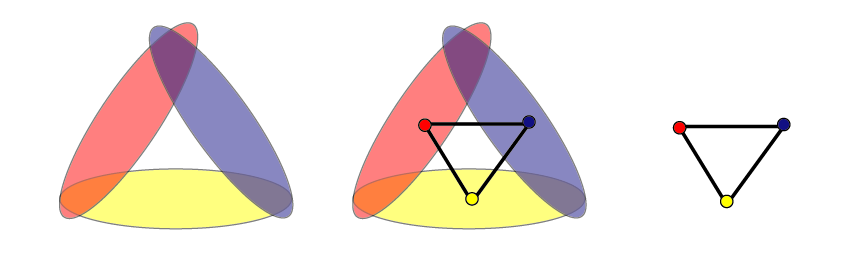
Let $𝒫$ be four points in ${ℝ}^2$ as in the figure.

The Čech complex created using $r=2$ is 1-dimensional – three of the points are linked.

The Čech complex created using $r=5$ is 2-dimensional – the three linked points now span a 2-simplex. The fourth point is also connected.

Homotopy type

05 Theory - Homotopy type and homology

Homology can be used to distinguish topological spaces or to measure the topological complexity of a space. From the perspective of computational complexity theory, homology is very easy to compute.

Theorem: Homology depends functionally on $|𝒦|$

The isomorphism types of the homology groups $H_i(𝒦;\mathbb{Z})$ of a simplicial complex $𝒦$ depend only on $|𝒦|$, the underlying topological space.

More precisely, a homeomorphism of topological spaces induces an isomorphism of homology groups.

This theorem implies that any two homeomorphic spaces have isomorphic homology groups.

• %& For a topological space $X$, we write $H_i(X;\mathbb{Z})$ for the homology groups of $X$ computed using any simplicial complex structure provided on $X$.
  • If $X$ does not have a simplicial complex structure, or $\mathrm{\Delta }$-complex structure, one can still define singular homology for $X$, and this homology still depends functionally only on the homeomorphism type.
  • Singular homology is isomorphic to simplicial and $\mathrm{\Delta }$-homology when the latter can be defined.

---

There is an equivalence relation between spaces that is much ‘coarser’ than homeomorphism, namely homotopy equivalence.

Homotopy equivalence

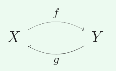
A homotopy equivalence between topological spaces $X$ and $Y$ is a pair $(f,g)$ of continuous maps:

such that $f\circ g$ is homotopic to ${\mathrm{Id}}_X$ and $g\circ f$ is homotopic to ${\mathrm{Id}}_Y$.

We write $X\simeq Y$ when $X$ and $Y$ are homotopy equivalent.

A homotopy from $f\circ g$ to ${\mathrm{Id}}_X$ would be a continuous map $F:X\times [\mathrm{0,1}]\to X$ such that $F(x,0)=(f\circ g)(x)$ and $F(x,1)={\mathrm{Id}}_X(x)=x$. Analogously for a homotopy $g\circ f$ to ${\mathrm{Id}}_Y$.

A homeomorphism is actually the special case of a homotopy equivalence where the homotopies $f\circ g\stackrel{\sim }{⟶}{\mathrm{Id}}_X$ and $g\circ f\stackrel{\sim }{⟶}{\mathrm{Id}}_Y$ are both the identity maps.

Theorem: Homology depends functionally on homotopy type

The isomorphism types of the homology groups $H_i(𝒦;\mathbb{Z})$ of a topological space $|𝒦|$ depend only on the homotopy type of the space.

More precisely, a homotopy equivalence of topological spaces induces an isomorphism of homology groups.

We will see a partial justification of this fact later, after discussing simplicial maps and chain maps.

Contractible spaces

A topological space is contractible if it is homotopy equivalent to a point.

06 Illustration

Contractibility of ${ℝ}^n$

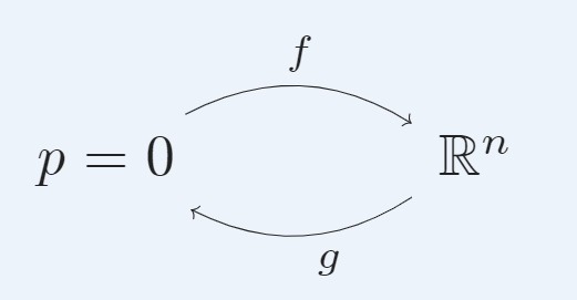
We show that ${ℝ}^n$ is contractible.

Let $p=0\in {ℝ}^n$ be the origin. Consider the maps $f$ and $g$:

Then $f\circ g:{ℝ}^n\to p$ is the constant map sending everything in ${ℝ}^n$ to the origin.

Define $F(x,t)=tx$. Then $F(x,0)\equiv 0$, which agrees with $f\circ g$, while $F(x,1)=x={\mathrm{Id}}_{{ℝ}^n}$. Therefore $f\circ g$ is homotopic to ${\mathrm{Id}}_{{ℝ}^n}$.

Now consider that $g\circ f={\mathrm{Id}}_p$ already. No additional homotopy is needed.

The same homotopy formula, namely $F(x,t)=tx$, can be used to show that any ball in ${ℝ}^n$ is contractible, and indeed any convex set in ${ℝ}^n$ is contractible.

• ! Therefore, any simplex is contractible.

Cylinder is homotopic to circle

A cylinder is given by $X={𝕊}^1\times [-\mathrm{1,1}]$. Consider the ‘collapse’ map $f:X\to {𝕊}^1$ given by projecting to the circle along straight lines, and the map $g:{𝕊}^1\hookrightarrow X$ given by inclusion:

The map $f\circ g$ is equal to the collapse map, and the map $g\circ f$ is the identity on ${𝕊}^1$.

Now construct a homotopy from the collapse map to ${\mathrm{Id}}_X$:

$$\begin{array}{cc}F:X\times [\mathrm{0,1}]& ⟶X\\ & \\ F:({𝕊}^1\times [-\mathrm{1,1}])\times [\mathrm{0,1}]& ⟶{𝕊}^1\times [-\mathrm{1,1}]\\ & \\ ((x,h),t)& ⟼(x,th)\end{array}$$

Rank of homology

07 Theory - Betti numbers, Euler Characteristic

Rank of an abelian group

Every finitely generated abelian group $G$ is isomorphic to a group with this form:

$${\mathbb{Z}}^r⨁\left({\oplus ︎}_i\mathbb{Z}/k_i\mathbb{Z}\right)$$

• The ${\mathbb{Z}}^r$ summands give a free abelian part and contain all infinite-order generators.
• The $\mathbb{Z}/k_i\mathbb{Z}$ summands give torsion and contain all finite-order generators.

The rank of $G$ is the number $r$.

Betti numbers

The Betti numbers ${\beta }_i$ of a topological space $X$ are the ranks of the homology groups:

$${\beta }_i(X)=\mathrm{rank}(H_i(X;\mathbb{Z}))$$

These Betti numbers may be combined into a single number, the Euler characteristic:

Euler characteristic

The Euler characteristic $\chi (X)$ of a topological space $X$ is the alternating sum of Betti numbers:

$$\chi (X)=\sum _i{(-1)}^i{\beta }_i(X)$$

08 Illustration

For convex polyhedra, Euler’s formula for the Euler characteristic is simply vertices minus edges plus faces:

$$\chi =V-E+F$$

For nonconvex polyhedra, this formula can give values other than the actual Euler characteristic defined using Betti numbers.

Name	Figure	Vertices	Edges	Faces	$\chi =V-E+F$
Tetrahedron		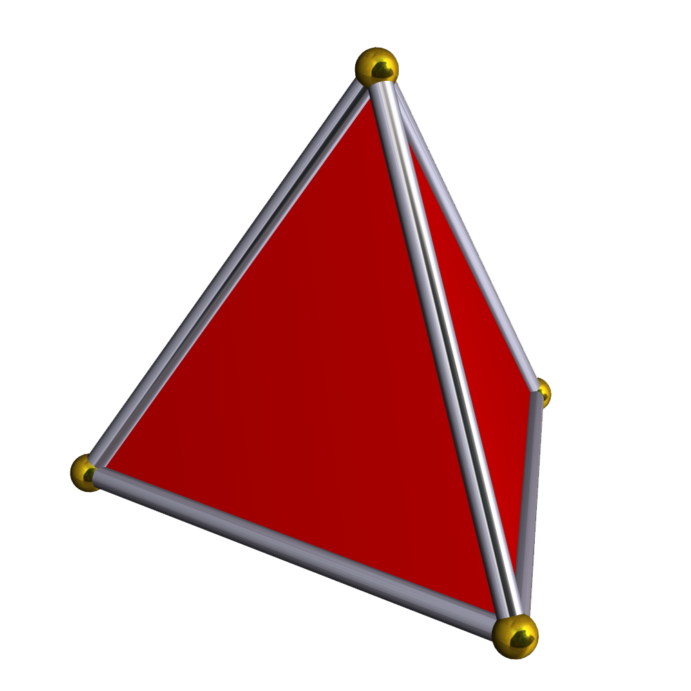4	6	4	2
Cube		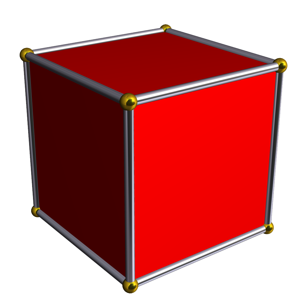8	12	6	2
Octahedron		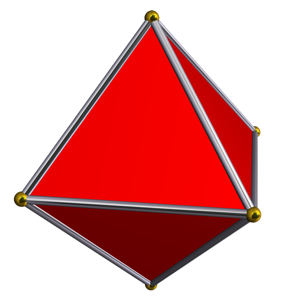6	12	8	2
Dodecahedron		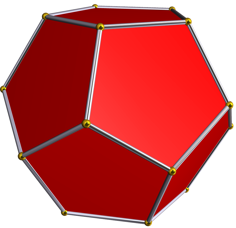20	30	12	2
Icosahedron		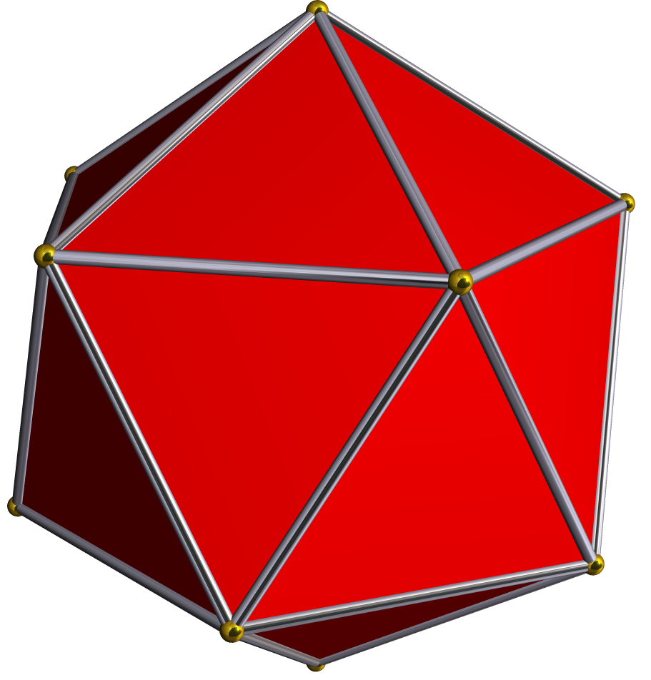12	30	20	2
Tetrahemihexahedron		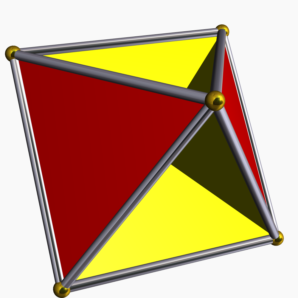6	12	7	1
Cubohemioctahedron		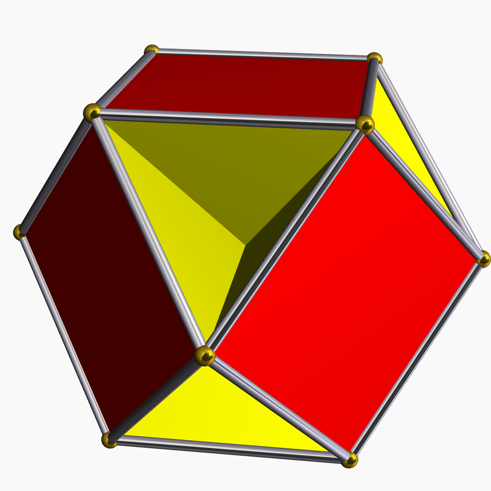12	24	10	-2
Small stellated dodecahedron		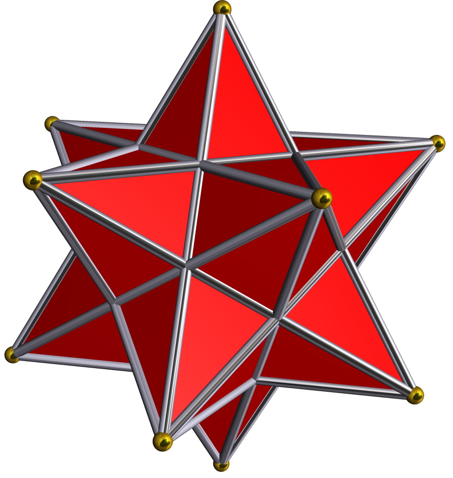12	30	12	-6

For a simplicial complex, the Euler characteristic can always be computed using a formula analogous to the Euler formula: count the simplices of each dimension:

$$\chi =k_0-k_1+k_2-k_3+\cdots \pm k_n$$

Here $k_i$ is the number of $i$-simplices in the simplicial complex.

Theorem: Euler $=$ Euler

For a simplicial complex, the same Euler characteristic may be calculated using Betti numbers or using the counts of simplices.

We do not prove this here, although the proof is a straightforward homology calculation.

Maps and homology

09 Theory - Simplicial maps, chain maps

Simplicial map

A map $f:𝒦\to ℒ$ between simplicial complexes is simplicial if it maps vertices of $𝒦$ to vertices of $ℒ$, and it maps simplices of $𝒦$ linearly to simplices of $ℒ$.

For example:

• Inclusions of one simplicial complex into another.
• Reduction of a simplicial complex to lower dimension, e.g. $[v_0,v_1]\to [v_0]$.

---

Chain map

A chain map $f$ is a map between chain complexes, which consists of a collection $f_n,\dots ,f_0$ of homomorphisms:

$$f_i:C_i(𝒦)\to C_i(ℒ)$$

of abelian groups which commute with the boundary operators:

$$f_{i-1}\circ {\partial }_i^{𝒦}={\partial }_i^{ℒ}\circ f_i\text{for all}i.$$

Such a chain map makes the following diagram commute:

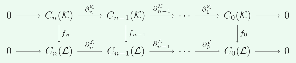
• The homomorphisms can be collected under a single map $f$, and the commutativity condition expressed simply:

$$f\circ {\partial }^{𝒦}={\partial }^{ℒ}\circ f$$

Theorem: Induced chain map

A simplicial map $f:𝒦\to ℒ$ determines a map of chain complexes $f:C(𝒦)\to C(ℒ)$.

The simplicial map $f$ is extended linearly from simplices to chains (from generators to linear combinations).

10 Theory - Induced maps on homology

Theorem: Induced map on homology

A chain map $f:𝒦\to ℒ$ determines a map $f_{\ast }$ of homology groups which splits by degrees:

$${f_{\ast }}_i:H_i(𝒦)\to H_i(ℒ)$$

A chain map $f$ sends cycles to cycles and boundaries to boundaries, so it descends to a map of quotient groups.

Proof of Theorem: Induced map on homology

It is sufficient to check that $f$ maps cycles to cycles and boundaries to boundaries:

• By mapping boundaries to boundaries, $f$ is well-defined on homology groups.
• By mapping cycles to cycles, $f$ maps elements of homology to elements of homology.

---

Checking $f$ maps cycles to cycles:

If $\tau \in \mathrm{Im}{\partial }^{𝒦}$, meaning that $\tau$ is a cycle, then $\tau ={\partial }^{𝒦}(\sigma )$ for some $\sigma$, whence:

$$\tau =(f\circ {\partial }^{𝒦})(\sigma )\text{⨠}\text{⨠}\tau =({\partial }^{ℒ}\circ f)(\sigma ),$$

but this implies $\tau \in \mathrm{Im}{\partial }^{ℒ}$.

---

Checking $f$ maps boundaries to boundaries:

If ${\partial }^{𝒦}(\tau )=0$, then:

$$\begin{array}{c}{\partial }^{ℒ}(f(\tau ))\text{⨠}\text{⨠}({\partial }^{ℒ}\circ f)(\tau )\text{⨠}\text{⨠}(f\circ {\partial }^{𝒦})(\tau )\\ \\ \text{⨠}\text{⨠}f({\partial }^{𝒦}(\tau ))\text{⨠}\text{⨠}f(0)\text{⨠}\text{⨠}0\end{array}$$

but this means the image of $\tau$ is a cycle.

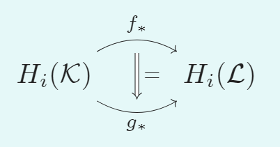
Proposition: Homotopic maps are the same on homology

If two maps of simplicial complexes $f,g:𝒦\to ℒ$ are homotopic, then they induce the same maps on homology groups, $f_{\ast }=g_{\ast }$:

In words: continuous deformations do not change the map induced on homology.

Proposition: Homology respects composition of maps

Given a composition of simplicial maps:

$$𝒦\stackrel{f}{⟶}ℒ\stackrel{g}{⟶}ℳ,$$

the map induced by the composite agrees with the composite of the induced maps:

$${(g\circ f)}_{\ast }=g_{\ast }\circ f_{\ast }:H_i(𝒦)\to H_i(ℳ)$$

The property of respecting composition of maps is called functoriality.

Corollary: Homotopy equivalence implies homology isomorphism

Homotopy equivalent simplicial complexes have isomorphic homology groups:

$$𝒦\simeq ℒ⟹H_i(𝒦)\cong H_i(ℒ)\text{for all}i$$

Proof of Corollary

Suppose we have a homotopy equivalence:

$$\begin{array}{c}𝒦\stackrel{f}{⟶}ℒ,ℒ\stackrel{g}{⟶}𝒦\\ \\ g\circ f\simeq {\mathrm{Id}}_{𝒦},f\circ g\simeq {\mathrm{Id}}_{ℒ}\end{array}$$

Now apply functoriality to the induced maps on homology:

$$\begin{array}{c}{g}_{\ast }\circ f_{\ast }\text{⨠}\text{⨠}{(g\circ f)}_{\ast }\text{⨠}\text{⨠}{({\mathrm{Id}}_{𝒦})}_{\ast }={\mathrm{Id}}_{H_i(𝒦)}\\ \\ f_{\ast }\circ g_{\ast }\text{⨠}\text{⨠}{(f\circ g)}_{\ast }\text{⨠}\text{⨠}{({\mathrm{Id}}_{ℒ})}_{\ast }={\mathrm{Id}}_{H_i(ℒ)}\end{array}$$

Therefore $g_{\ast }$ is the inverse of $f_{\ast }$ as homomorphisms of abelian groups.

11 Illustration

Contraction to a point

The map $f:{ℝ}^n\to \{p\}$ for some point $p\in {ℝ}^n$ is a homotopy equivalence, so it induces an isomorphism on homology. Therefore:

$$H_i({ℝ}^n)=\{\begin{array}{cc}0& i>0\\ \mathbb{Z}& i=0\end{array}$$

Dunce Hat

The Dunce Hat is formed by identifying all sides of a triangle with non-circular identifications:

The Dunce Hat is contractible, but it is not collapsible. The contraction can be performed by embedding the Hat in a 3-ball in ${ℝ}^4$.

Because it is contractible, the Dunce Hat has the homology of a point.

Homology of a cylinder

Recall that the cylinder is homotopic to the circle (§06):

A circle is homeomorphic to a triangle.

We have computed the homology of a triangle (§11 of Part I).

Therefore the homology of the cylinder is:

$$H_i(X)=\{\begin{array}{cc}0& i>2\\ \mathbb{Z}& i=1\\ \mathbb{Z}& i=0\end{array}$$

Homology variations

12 Theory - Relative homology

Suppose a simplicial complex $𝒦$ is embedded within another simplicial complex $ℒ$. The homology of $ℒ$ relative to $𝒦$ is given by zeroing (quotienting out) the cycles fully within $𝒦$. Only cycles that inescapably involve $ℒ$ outside of $𝒦$ contribute to the relative homology.

More precisely, suppose that $𝒦\subset ℒ$, so vertices and simplices of $𝒦$ are also vertices and simplices of $ℒ$.

Then observe that chains in $𝒦$ are automatically chains in $ℒ$, and thus:

$$𝒦\subset ℒ⟹C_i(𝒦)<C_i(ℒ)\text{for all}i$$

(A subgroup: because a sum of chains in $𝒦$ is still a chain in $𝒦$.)

Relative chain complex

Suppose $𝒦\subset ℒ$ is an inclusion of simplicial complexes.

Define $C_i(ℒ,𝒦)$, the relative chain group, as the quotient:

$$C_i(ℒ,𝒦)=\frac{C_i(ℒ)}{C_i(𝒦)}$$

Proposition: Boundary maps descend to relative chain groups

The boundary maps $\partial :C_i(ℒ)\to C_{i-1}(ℒ)$ send chains in $𝒦$ to chains in $𝒦$ and thus descend to the quotient groups, giving a relative chain complex:

$$0\to C_n(ℒ,𝒦)\stackrel{{\partial }^{ℒ,𝒦}}{⟶}\cdots \stackrel{{\partial }^{ℒ,𝒦}}{⟶}{C}_0(ℒ,𝒦)\to 0$$

(Here ${\partial }^{ℒ,𝒦}$ is just the map induced by $\partial$ on the quotient groups.)

Proof of Proposition: Boundary maps descend to relative chain groups

It is sufficient to establish that boundaries from $𝒦$ must also reside in $𝒦$, i.e. that:

$$\partial (C_i(𝒦))\subset C_{i-1}(𝒦)$$

But this is clear because $𝒦$ is a simplicial complex, so it is closed under taking boundaries.

Relative homology

Suppose $𝒦\subset ℒ$ is an inclusion of simplicial complexes.

Define $H_k(ℒ,𝒦)$, the relative homology group, as the homology group of the relative chain complex:

$$H_k(ℒ,𝒦)=\frac{\mathrm{Ker}\left({\partial }_k^{ℒ,𝒦}\right)}{\mathrm{Im}\left({\partial }_{k+1}^{ℒ,𝒦}\right)}$$

Remark: Relativizing before homology

It is tempting to try relativizing the homology groups directly.

The inclusion $𝒦\hookrightarrow ℒ$ does induce maps $H_k(𝒦)\to H_k(ℒ)$. We could study the groups $H_k(ℒ)/H_k(𝒦)$.

These quotient groups are not what relative homology is after! See the illustrations.

13 Illustration

Homology of a simplex relative to its boundary

Consider a simple 2-simplex $\sigma$ and the simplicial complex $ℒ$ that it determines:

Let $𝒦$ be the boundary 1-simplex (the edges only from $ℒ$).

There are no 2-simplices in $𝒦$, so:

$$C_2(ℒ,𝒦)=C_2(ℒ)\cong ⟨\sigma ⟩\cong \mathbb{Z}$$

All 0- and 1-simplices in $ℒ$ are also in $𝒦$, so:

$$C_1(ℒ,𝒦)=0,C_0(ℒ,𝒦)=0$$

The relative chain complex:

$$0\to C_2(ℒ,𝒦)\to C_1(ℒ,𝒦)\to C_0(ℒ,𝒦)\to 0$$

becomes:

$$0\to \mathbb{Z}\to 0\to 0\to 0$$

It follows that the relative homology is:

$$H_i(ℒ,𝒦)=\{\begin{array}{cc}0& i>3\\ \mathbb{Z}& i=2\\ 0& i=1\\ 0& i=0\end{array}$$

Compare this to the homology of a sphere!

Homology of a sphere:

$$H_i({𝕊}^2)=\{\begin{array}{cc}0& i>3\\ \mathbb{Z}& i=2\\ 0& i=1\\ \mathbb{Z}& i=0\end{array}$$

Notice that ${𝕊}^2$ is homeomorphic to the quotient space $ℒ/𝒦$.

This comparison of homologies is apt; we just need to explain $H_0({𝕊}^2)\cong \mathbb{Z}$ versus $H_0(ℒ,𝒦)\cong 0$.

Compare this against the quotient of homology groups!

The homology of $𝒦$ is:

$$H_i(𝒦)=\{\begin{array}{cc}0& i>1\\ \mathbb{Z}& i=1\\ \mathbb{Z}& i=0\end{array}$$

The homology of $ℒ$, because it is contractible, is:

$$H_i(ℒ)=\{\begin{array}{cc}0& i>0\\ \mathbb{Z}& i=0\end{array}$$

The quotient of homology groups is:

$$H_i(ℒ)/H_i(𝒦)\cong 0\text{for all}i$$

• Relative homology treats $𝒦$ as a single point.
• The quotient of homology annihilates generators (“holes”) in $ℒ$ which are also generators (“holes”) in $𝒦$.
• Different results for different constructions!

14 Theory - Cochain complex

Recall that the chain group $C_k(𝒦)$ is the free abelian group of formal linear combinations of $k$-simplices in $𝒦$:

$$C_k(𝒦)=\{\sum _{i\in I\text{finite}}{n}_i{\sigma }_i|n_i\in \mathbb{Z},{\sigma }_i\in 𝒦,\dim ({\sigma }_i)=k\}$$

One should think of the chains $\sum n_i{\sigma }_i$ as assignments of integers $n_i$ to the various $k$-simplices in $𝒦$.

Thinking in this way, the boundary map ${\partial }_k:C_i\to C_{i-1}$ is given on chains by simple linear extension of its definition for individual simplices. Thus ${\partial }_k\left(n_i{\sigma }_i\right)=n_i{\partial }_k({\sigma }_i)$.

---

Cohomology is created by interpreting the integers $n_i$ not as coefficients, but as the outputs of linear functions $C_k\to \mathbb{Z}$.

To notate this effectively, define indicator functions ${\phi }_i$ for each of the $k$-simplices:

$$\begin{array}{c}{\phi }_i:\{\text{oriented }k\text{-simplices in }𝒦\}\to \mathbb{Z}\\ \\ {\sigma }_i\mapsto 1,{\sigma }_j\mapsto 0\text{for}j\ne i\end{array}$$

Cochains

The space of linear maps $C_k\to \mathbb{Z}$ is isomorphic to the free abelian group of formal linear combinations of indicator functions:

$$C^k(𝒦)=\{\sum _{i\in I}{m}_i{\phi }_i|m_i\in \mathbb{Z},{\phi }_i\text{indicator of}{\sigma }_i\}$$

Elements of this space, written generically as formal sums $m_1{\phi }_1+m_2{\phi }_2+\cdots$, are called cochains.

(For cochains it is not necessary that $I$ be finite.)

Since there is a bijective correspondence of sets between oriented simplices and their indicator functions, we see that $C^k(𝒦)\cong C_k(𝒦)$ as abelian groups; we have simply reinterpreted the chains as assignments of integers $m_i$ to the indicators of $k$-simplices in $𝒦$.

---

In both cases, the data of a chain / cochain consists of the assignment of a number ($n_i$ or $m_i$) to each of the $k$-simplices in $𝒦$. But the difference in interpretation of this data allows a difference in the construction of boundary operators:

Coboundary operator

Define the coboundary operator thus:

$$\begin{array}{cc}{\delta }^k:C^k(𝒦)& \to C^{k+1}(𝒦)\\ & \\ {\phi }_i& \mapsto {\phi }_i\circ {\delta }^{k+1}(\text{extended linearly})\end{array}$$

In words: the coboundary of a simplex indicator indicates that simplex in the boundary of a higher simplex.

For example, in the triangular 2-simplex:

If ${\phi }_{[v_0,v_2]}$ is the indicator of $[v_0,v_2]$, then the coboundary ${\delta }^1\left({\phi }_{[v_0,v_2]}\right)$ indicates the presence of $[v_0,v_2]$ in the boundaries of 2-simplices. It returns $-1$ for the triangle itself, $[v_0,v_1,v_2]$, since the boundary of the triangle includes the term $-[v_0,v_2]$.

Thus, in general, ${\delta }^k\left(m_i{\phi }_i\right)=m_i({\phi }_i\circ {\partial }_k)$, in contrast to ${\partial }_k\left(n_i{\sigma }_i\right)=n_i{\partial }_k({\sigma }_i)$ that we saw for ${\partial }_k$.

---

Witness a simple computation, applying ${\delta }^{k+1}\circ {\delta }^k$ to an arbitrary indicator:

$$\begin{array}{c}({\delta }^{k+1}\circ {\delta }^k)({\phi }_i)\text{⨠}\text{⨠}{\delta }^{k+1}({\delta }^k({\phi }_i))\\ \\ \text{⨠}\text{⨠}{\delta }^{k+1}({\phi }_i\circ {\partial }_k)\text{⨠}\text{⨠}{\phi }_i\circ {\partial }_k\circ {\partial }_{k+1}\text{⨠}\text{⨠}0\end{array}$$

Cochain complex

Given a simplicial (or $\mathrm{\Delta }$-) complex $𝒦$ of maximal dimension $n$, we define the cochain complex of $𝒦$ as the sequence of morphisms:

$$0⟵C_n\stackrel{{\delta }^{n-1}}{⟵}{C}_{n-1}\stackrel{{\delta }^{n-2}}{⟵}{C}_{n-2}⟵\cdots ⟵C_1\stackrel{{\delta }^0}{⟵}{C}_0⟵0$$

This sequence is a complex because:

$${\delta }^{k+1}\circ {\delta }^k=0\text{for every}k$$

The image and kernel groups are named in the obvious way:

• $B_k:=\mathrm{Im}({\delta }^{k-1})$ — called the coboundary cochains
• $Z_k:=\mathrm{Ker}({\delta }^k)$ — called the cocycles

15 Theory - Cohomology

Cohomology

The $k^{\text{th}}$ cohomology of $𝒦$ is defined as the quotient group of cocycles modulo coboundary chains:

$$H^k(𝒦)=\frac{\mathrm{Ker}({\delta }^k)}{\mathrm{Im}({\delta }^{k-1})}$$

---

Cohomology is an upgrade from homology because it has an additional product structure, so cohomology actually gives a collection of rings.

Cup product on cochains, for simplicial complexes

Suppose we are given a simplicial complex $𝒦$, together with a chosen ordering $O=(v_1,\dots ,v_N)$ of all vertices of $𝒦$.

There are maps of cochain groups $C^k\times C^{\ell }\to C^{k+\ell }$ defined as follows:

For any pair of cochains $\phi \in C^k$ and $\psi \in C^{\ell }$, and any vertices $w_0<\cdots <w_{k+\ell }$ ordered according to $O$, with $[w_0,\dots ,w_{k+\ell }]$ the $(k+\ell )$-simplex they form, we have:

$$(\phi ⌣\psi )([w_0,\dots ,w_{k+\ell }])=\phi ([w_0,\dots ,w_k])\cdot \psi ([w_k,\dots ,w_{k+\ell }])$$

Note: the oriented simplices here may be written with various orderings, but the splitting into $k$- and $\ell$-simplices must follow the order of $O$.

Cup product using indicators

Let $\phi \in C^k$ be the indicator of an oriented simplex $[u_{i_0},\dots ,u_{i_k}]$, and let $\psi \in C^{\ell }$ be the indicator of another oriented simplex $[v_{i_k},\dots ,v_{i_{k+\ell }}]$.

Let $(w_0,\dots ,w_{k+\ell })$ be the vertices of the total list

$$u_{i_0},\dots ,u_{i_k},v_{i_k},\dots ,v_{i_{k+\ell }}$$

reordered in the ordering of $O$ (allowing repetition), so $w_0\le w_1\le \cdots \le w_{k+\ell }$.

Then $\phi ⌣\psi$ is defined as follows: it is the indicator of $[w_0,\dots ,w_{k+\ell }]$ provided:

• (i) the $w_i$ are all distinct,
• (ii) $u_p\le v_q$ for all $p,q$;

and $\phi ⌣\psi =0$ if (i) and (ii) do not hold.

The definition is extended bilinearly to all of $C^k\times C^{\ell }$.

Vertex orderings and the cup product

Instead of choosing a total ordering $O$ of all vertices of $𝒦$, it is sufficient to choose a partial ordering of the vertices $v_1,\dots ,v_N$ of $𝒦$ having the property that $O$ induces a total ordering of each simplex of $𝒦$.

A set of compatible orderings of the vertices in each simplex is used to define a ‘front half’ and ‘back half’ of each $(k+\ell )$-simplex $\sigma$, thereby cutting $\sigma$ into one $k$-simplex and one $\ell$-simplex.

The cutting method applied to a given simplex must be compatible with the method applied to every other simplex. A global vertex ordering ensures this compatibility.

Cup product on cohomology

The cup product has the following relation to the coboundary operator, a type of signed Leibniz rule:

$$\delta (\phi ⌣\psi )=\delta \phi ⌣\psi +(-1{)}^k\phi ⌣\delta \psi$$

when $\phi \in C^k(𝒦)$.

This formula implies that if $\phi$ and $\psi$ are cocycles (or coboundaries), then $\phi ⌣\psi$ is also a cocyle (coboundary). Therefore the cup product descends to cohomology:

$$H^k(𝒦)\times H^{\ell }(𝒦)\to H^{k+\ell }(𝒦)$$

The cup product on cohomology provides a ring structure to the direct sum ${⨁}_i{H}^i(𝒦)$. The product, and the ring structure, do not depend on the choice of ordering used to define the product on cochains.

(Note: The cup product is always zero when $k+\ell$ is greater than the maximal simplex dimension.)

16 Illustration

Some cohomology classes on the 2-torus

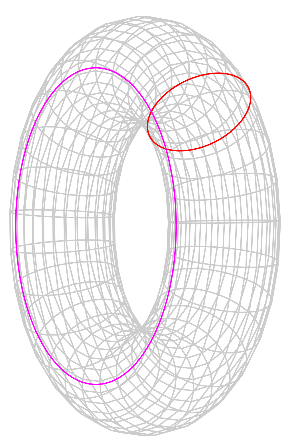
Consider the 2-torus $T$:

The red (poloidal) and pink (toroidal) curves together generate the degree one homology, $H_1(T)\cong {\mathbb{Z}}^2$.

Now recall a simplicial complex representation of the torus:

Let $\phi$ be the cochain which assigns 1 to every edge in the middle column, and zero to all other edges. (So it is 1 on the edges directly below the $\phi$ label, including the diagonals, but excluding all verticals.) Let $\psi$ be the cochain which assigns 1 to every edge in the middle row, and zero to all other edges. (So it is 1 on the edges directly to the right of the $\psi$ label, including the diagonals, but excluding all horizontals.) Accounting now for orientations, let $\phi$ give $+1$ on edges directed rightwards, and $\psi$ give $+1$ on edges directed upwards.

One can check directly, going around the boundaries of each 2-simplex, that $\delta \phi =0$ and $\delta \psi =0$: The sum of the numbers on any triangle, accounting for orientations, is zero. So these cochains are both cocycles.

In order to see that $\phi$ and $\psi$ are not boundaries, and thus represent nontrivial homology classes, and also to see that they don’t represent the same homology class, we devise a method of representing coboundaries of 0-cochains.

A 0-cochain $\eta$ is the assignment of integers to each of the vertices. The condition $\delta \eta =0$, which means $\eta \circ {\partial }_1\equiv 0$, states that these numbers cannot change as one moves across an edge from vertex to vertex. (Applying ${\partial }_1$ to any edge $[u,v]$ gives $[v]-[u]$. By linearity, $\eta ({\partial }_1([u,v]))=\eta ([v])-\eta ([u])$. Therefore $\eta ([v])=\eta ([u])$ when the condition holds.)

From this it follows that $H^0(T)\stackrel{\sim }{⟶}\mathbb{Z}$. The isomorphism is given by sending $\eta$ to the integer it gives on a vertex.

Return now to $H^1(T)$. A boundary in $H^1(T)$ is a cochain $\chi$ assigning numbers to directed edges such that there is a vertex labeling cochain $\eta \in C^1$ with $\chi ([u,v])=\eta ([v])-\eta ([u])$. In other words, that it is possible to derive the edge numbers as the differences of a single vertex numbering scheme.

Now one can see that $\phi$ is not a coboundary. Vertex integers must increase by one as one passes across the middle column of edges, and stay fixed going across all other edges. This is impossible because the left-most and right-most edges are identified. Similarly $\psi$ is not a coboundary, and $\phi -\psi$ is not a coboundary.

(To witness a contrasting case, let $\xi$ be a 1-cochain giving 1 only on the non-vertical edges in the right-most column. This is $\phi$ shifted to the right. Now $\phi -\xi$ is a coboundary: assign 1 on vertices in the middle-right column, and 0 on all other vertices.)

Much more work would be required to show that $\phi$ and $\psi$ have no relations in homology, and that they jointly generate homology.

A cup product on the 2-torus

We study the cup product $\phi ⌣\psi$:

We must provide an ordering $O$ of all the vertices of the torus. Order them as in a book: top-to-bottom, then left-to-right.

Let us see how to verify the values on the green and yellow 2-simplices. Label the vertices of the inner square as in the figure; the index ordering is compatible with $O$.

For the green 2-simplex $[v_0,v_1,v_2]$, we have $\phi ([v_0,v_1])=+1$ and $\psi ([v_1,v_2])=-1$, so:

$$(\phi ⌣\psi )([v_0,v_1,v_2])=(+1)\cdot (-1)=-1$$

For the yellow 2-simplex $[v_1,v_2,v_3]$, we have $\phi ([v_1,v_2])=-1$ and $\psi ([v_2,v_3])=0$, so:

$$(\phi ⌣\psi )([v_1,v_2,v_3])=(+1)\cdot (0)=0$$

A calculation with more details (illustrating bilinearity) can be performed in terms of the indicator functions. Write:

$$\phi ={\phi }_1+\cdots +{\phi }_6,\psi ={\psi }_1+\cdots +{\psi }_6$$

where ${\phi }_i$ is the indicator for the edge in the support of $\phi$ which is in the $i^{\text{th}}$ place from the top (oriented rightwards), and analogously ${\psi }_j$ is for the one for $\psi$ in the $j^{\text{th}}$ place from the left (oriented upwards).

Applying bilinearity to expand the cup product:

$$\begin{array}{c}\phi ⌣\psi \text{⨠}\text{⨠}({\phi }_1+\cdots +{\phi }_6)⌣({\psi }_1+\cdots +{\psi }_6)\\ \text{⨠}\text{⨠}\sum _{i=1}^6\sum _{j=1}^6{\phi }_i⌣{\psi }_j\end{array}$$

The edges with indicators ${\phi }_i$ and ${\psi }_j$ could span one of the 2-simplices only when $i=3,4,5$ and $j=3,4,5$. And in fact the pairs $(i,j)=(\mathrm{3,5}),(\mathrm{5,3})$ can be ruled out as well. The only terms to consider are these six:

$$\begin{array}{c}\sum _{i=1}^6\sum _{j=1}^6{\phi }_i⌣{\psi }_j\text{⨠}\text{⨠}\begin{array}{c}{\phi }_3⌣{\psi }_3+{\phi }_3⌣{\psi }_4+{\phi }_4⌣{\psi }_3\\ +{\phi }_4⌣{\psi }_5+{\phi }_5⌣{\psi }_4+{\phi }_5⌣{\psi }_5\end{array}\end{array}$$

• Now ${\phi }_3$ is the indicator for $[v_0,v_1]$ and ${\psi }_3$ is the indicator for $[v_0,v_2]$, so ${\phi }_3⌣{\psi }_3=0$ because $v_1\nleqq v_0$ so the total list $v_0,v_1,v_0,v_2$ does not split according to the ordering of $O$.
• Then ${\psi }_4$ is the indicator for $-[v_1,v_2]$, so ${\phi }_3⌣{\psi }_4$ is the indicator for $-[v_0,v_1,v_2]$, meaning it returns $-1$ on the green 2-simplex.
• Then ${\phi }_4$ is the indicator for $-[v_1,v_2]$, so ${\phi }_4⌣{\psi }_3=0$.
• Then ${\psi }_5$ is the indicator for $-[v_1,v_3]$, so ${\phi }_4⌣{\psi }_5=0$ because $v_2\nleqq v_1$.
• Then ${\phi }_5$ is the indicator for $[v_2,v_3]$, so ${\phi }_5⌣{\psi }_4=0$ because $v_2\nleqq v_1$.
• Then ${\phi }_5⌣{\psi }_5=0$ as well, also because $v_2\nleqq v_1$.

By adding these results, we see that $\phi ⌣\psi$ is the indicator for the central 2-simplex, oriented clockwise.

This cochain in $C^2$ is automatically a cocycle because $C^3$ is empty.

Is it a coboundary?

To see that the answer is “no,” we can devise another scheme to represent coboundaries, now for $2$-simplices. We give here only a sketch. Give a 1-cochain $\xi$ which assigns integers to the edges. Draw oriented paths crossing the edges, with the number of paths crossing $e_i$ matching $\xi (e_i)$. Then $\delta \xi (t_j)$ for a triangle $t_j$ counts the total flow of paths into or out from $t_j$; it is a ‘sink’ or ‘source’ number describing extra paths originating or terminating inside $t_j$. The condition $\delta \xi (t_j)=0$ would mean that the paths are conserved in $t_j$, none created or destroyed.

With this perspective, it is obvious that the cochain $\phi ⌣\psi$ depicted in the figure cannot be a coboundary. Every 2-cochain which is a coboundary describes a collection of oriented paths that are created or destroyed only in triangles with nonzero assignments, according to that assignment. So $\phi ⌣\psi$ would describe a single path terminating in the green triangle, but originating nowhere, since there is no other sink or source.

Another observation is worth making about $\phi ⌣\psi$. It is the generator of $H^2(T)$.

Note that the full cohomology of $T$ is given by:

$$H^i(T)\cong \{\begin{array}{cc}0& i>3\\ \mathbb{Z}& i=2\\ {\mathbb{Z}}^2& i=1\\ \mathbb{Z}& i=0\end{array}$$

Here is a fact: All indicator functions on 2-simplices determine the same cohomology class. To see this, take the difference of any two indicators. Draw a simple oriented path out of one of them into the other. This path will define a 1-cochain by assigning $\pm 1$ on any edge it crosses on the way (according to their mutual orientations), and 0 on all edges it does not cross. The coboundary of this cochain gives $+1$ on the triangle from which the path emanates, and $-1$ on the triangle in which the path terminates, and zero on all other triangles. That is exactly the difference of indicator 2-simplices we started with.

Since $H^2(T)$ is generated by indicator 2-simplices, and they are all equivalent, we deduce that it is generated by $\phi ⌣\psi$.

To see that it is in fact infinite and isomorphic to $\mathbb{Z}$, we must exclude relations among the multiples of $\phi ⌣\psi$. A relation $n(\phi ⌣\psi )=m(\phi ⌣\psi )$ is equivalent to the relation $\ell (\phi ⌣\psi )=0$ for $\ell =n-m$. But we can exclude any such relation by the reasoning used above: a cochain $\ell (\phi ⌣\psi )$ cannot be a coboundary because it would represent $\ell$ oriented paths terminating in the green 2-simplex, and originating nowhere.

Therefore we have proven that:

$$H^2(T)\cong ⟨[\phi ⌣\psi ]⟩\cong \mathbb{Z}$$

The cocycle $[\phi ⌣\psi ]$ is called the fundamental cocycle of $T$.

Cohomology ring has topological significance

Let $X={𝕊}^1\times {𝕊}^1$, the 2-torus.

Let $Y={𝕊}^1\vee {𝕊}^1\vee {𝕊}^2$, a 2-sphere with two circles attached at one common point.

The cohomology groups are isomorphic:

$$H^i(X)\cong H^i(Y)\cong \{\begin{array}{cc}0& i>2\\ \mathbb{Z}& i=2\\ \mathbb{Z}\oplus ︎\mathbb{Z}& i=1\\ \mathbb{Z}& i=0\end{array}$$

However, the cup product operations differ, so the ring structures differ.

• In $X$, the cup product of the two generating cocycles is the fundamental coclass of the 2-torus.
• In $Y$, the cup product of the two generating cocycles (dual to the two copies of ${𝕊}^1$), is zero.

17 Theory - Coefficients

It is possible to define homology and cohomology with other coefficients. Given an abelian group $G$, one defines the chain groups thus:

$$C_k(𝒦,G)=\{\sum _{i\in I\text{finite}}{g}_i{\sigma }_i|g_i\in G,{\sigma }_i\in 𝒦,\dim ({\sigma }_i)=k\}$$

And the cochain groups thus:

$$C^k(𝒦,G)=\{\sum _{i\in I}{g}_i{\phi }_i|g_i\in \mathbb{Z},{\phi }_i\text{indicator of}{\sigma }_i\in 𝒦,\dim ({\sigma }_i)=k\}$$

Homology and cohomology are defined in the usual way from these chain groups.

The most important cases are $G=ℝ$ (which eliminates torsion), and $G=\mathbb{Z}/2\mathbb{Z}$ (where coefficients track parity only).

Manifolds

18 Theory - Topological and smooth manifolds

Topological manifold

A (second-countable, Hausdorff) topological space $X$ is an $n$-dimensional (topological) manifold if every point $p\in X$ has an open neighborhood $U$ which is homeomorphic to ${ℝ}^n$.

$$\text{“ the local topology of an }n\text{-manifold is that of }{ℝ}^n\text{ ”}$$

Notes:

• An equivalent definition is that every $p$ has open neighborhood $U$ homeomorphic to the open ball ${𝔹}_1(0)\in {ℝ}^n$, since of course ${𝔹}_1(0)$ is itself homeomorphic to ${ℝ}^n$.
• It is a theorem that every $n$-manifold can be embedded in some Euclidean space ${ℝ}^N$, so an equivalent definition states adds the hypothesis that $X\subset {ℝ}^N$ for some $N$.

---

To define smooth manifolds, we must first define differentiable and smooth maps.

Regular points

Suppose $p\in V\subset {ℝ}^n$ with $V$ open. Let $(x_1,\dots ,x_n)$ give coordinates on ${ℝ}^n$.

Suppose $f:V\to {ℝ}^d$ is a function given in coordinates by $f(x_1,\dots ,x_n)=(f_1,\dots ,f_d)$.

The differential matrix of $f$ at $p=(x_1,\dots ,x_n)$ is the Jacobi matrix:

$$[d_{p}f]=\left(\begin{array}{ccc}{\displaystyle \frac{\partial f_1}{\partial x_1}(p)}& \cdots & {\displaystyle \frac{\partial f_1}{\partial x_n}(p)}\\ ⋮& \ddots & ⋮\\ {\displaystyle \frac{\partial f_d}{\partial x_1}(p)}& \cdots & {\displaystyle \frac{\partial f_d}{\partial x_n}(p)}\end{array}\right)$$

The point $p$ is regular for $f$ when $[df]$ has rank $n$. (No point can be regular when $d<n$.)

Smooth manifold in ${ℝ}^d$

A subspace $M\subset {ℝ}^d$ is a smooth $n$-manifold if every $p\in M$ has an open neighborhood in $M$ (open in the subspace topology) that is the image of a smooth injective function $\phi :U\to {ℝ}^d$, whose domain is an open set $U\subset {ℝ}^n$, and whose differential $[d\phi ]$ has maximal rank everywhere on $U$.

Each such function is called a parametrization or a coordinate chart for $M$, and the image of a parametrization is a coordinate patch on $M$.

---

A parametrized surface is a bijective and infinitely differentiable (smooth) injective map:

$$\phi :U\to {ℝ}^3$$

where the parameter domain $U$ is an open subset of ${ℝ}^2$. Every parametrized surface defines a $2$-manifold in ${ℝ}^3$.

Using coordinates $(x,y)$ on ${ℝ}^2$ and $({\phi }_1,{\phi }_2,{\phi }_3)$ for the images of $\phi$ in ${ℝ}^3$, we have for the differential matrix:

$$[d_{(x,y)}\phi ]=\left(\begin{array}{cc}{\displaystyle \frac{\partial {\phi }_1}{\partial x}}& {\displaystyle \frac{\partial {\phi }_1}{\partial y}}\\ {\displaystyle \frac{\partial {\phi }_2}{\partial x}}& {\displaystyle \frac{\partial {\phi }_2}{\partial y}}\\ {\displaystyle \frac{\partial {\phi }_3}{\partial x}}& {\displaystyle \frac{\partial {\phi }_3}{\partial y}}\end{array}\right)$$

The maximum rank of $[d\phi ]$ is $2$, and $\mathrm{Rank}[d\phi ]=2$ occurs when any of these equivalent conditions are satisfied:

• The columns of $[d\phi ]$ are linearly independent (for two columns: not collinear vectors)
• There are two linearly independent rows in $[d\phi ]$
• There is a $2\times 2$ submatrix of $[d\phi ]$ with nonzero determinant

If the matrix $[d\phi ]$ is considered as a linear map $[d\phi ]:{ℝ}^2\to {ℝ}^3$, then the image of $[d\phi ]$ at $p=(x,y)$ is a plane through the origin which is parallel to the tangent plane to the surface at $\phi (x,y)$.

The condition $\mathrm{Rank}[d\phi ]=2$ ensures that small movements in the parameter space, $dx$ and $dy$, can generate two dimensions of movement on the surface. In turn this ensures that locally around $\phi (x,y)$ the surface is homeomorphic to an open disk in ${ℝ}^2$, and moreover that such a homeomorphism can be constructed as projection to the tangent plane at $\phi (x,y)$ composed with a linear map.

19 Illustration

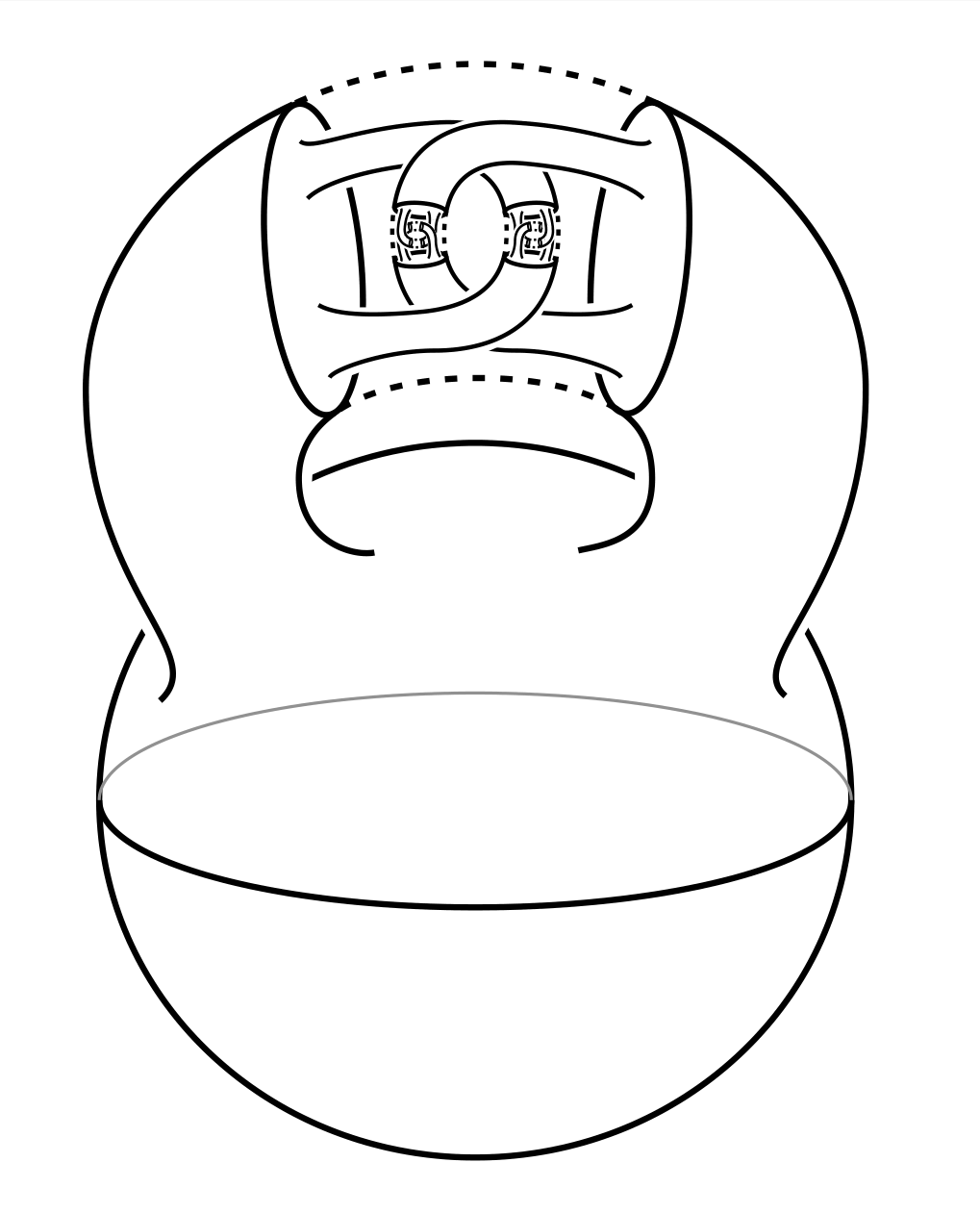
Wild topological manifolds

Topological spaces can be stranger than one imagines on the basis of simple examples. Here is Alexander’s Horned Sphere (/media/File:Construcción_de_esfera_de_Alexander_con_cuernos.gif; explanatory essay):

The horned sphere $S$ is a subset of ${ℝ}^3$ homeomorphic to ${𝕊}^2$. The outside ${ℝ}^3-S$ contains non-collapsible loops (so it is not simply connected), which is unlike the standard inclusion of ${𝕊}^2$ in ${ℝ}^3$.

The map $f:{𝕊}^2\hookrightarrow {ℝ}^3$ with $f({𝕊}^2)=S$ is an embedding of topological spaces and thus topological manifolds. (It is continuous, injective, and induces a homeomorphism onto the image which is endowed with the subspace topology; so the image is homeomorphic to ${𝕊}^2$ as a topological manifold.)

The map $f$ is not an embedding of differentiable, smooth, or piecewise linear manifolds.

Parametrized paraboloid

Let $\phi :{ℝ}^2\to {ℝ}^3$ by $\phi :(x,y)\mapsto (x,y,x^2+y^2)$.

Then $[d\phi ]$ is given by:

$$[d_{(x,y)}\phi ]=\left(\begin{array}{cc}1& 0\\ 0& 1\\ 2x& 2y\end{array}\right)$$

Notice that the determinant of the upper $2\times 2$ square is nonzero.

Singular curve

Consider $\phi :ℝ\to {ℝ}^2$ given by $\phi (t)=(t^2,t^3)$:

Then: $[d_t\phi ]=\left[\begin{array}{c}2t\\ 3t^2\end{array}\right]$ and $[d_0\phi ]=\left[\begin{array}{c}0\\ 0\end{array}\right]$.

Parametrized 2-sphere

Spherical coordinates define a parametrization of the 2-sphere:

$$f(\theta ,\phi )=(\sin \phi \cos \theta ,\sin \phi \sin \theta ,\cos \phi )$$

The differential:

$$[d_{(x,y)}\phi ]=\left(\begin{array}{cc}\cos \phi \cos \theta & -\sin \phi \sin \theta \\ \cos \phi \sin \theta & \sin \phi \cos \theta \\ -\sin \phi & 0\end{array}\right)$$

Notice that poles of the sphere correspond to points with $\phi =n\pi$, and there the right column is all zeros. So poles are not regular points of $\phi$. One can check that every other point is regular by computing the cross product of the column vectors.

Also, at the poles the function is not injective.

Therefore one must restrict the domain, for example to $\phi \in (-\pi ,\pi )$ and $\theta \in (\mathrm{0,2}\pi )$, to get a true parametrization. Unfortunately this does not cover the entire sphere; indeed it is impossible to cover the sphere with a single parametrization.

Parametrized 2-torus in ${ℝ}^4$

The 2-torus can be parametrized in ${ℝ}^4$ very easily:

$$f(\phi ,\theta )=(\cos \phi ,\sin \phi ,\cos \theta ,\sin \theta )\phi ,\theta \in (\mathrm{0,2}\pi )$$

This parametrization is regular everywhere, but the domain cannot be extended to cover the entire torus without becoming non-injective (and no longer a homeomorphism onto its image), for topological reasons. The torus cannot be covered by a single parametrization.