TDA Notes - Unit 03

Manifolds cont’d

01 Theory - Local coordinates

Smooth map

A map $\phi :U\to V$ for open sets $U\subset {ℝ}^n$ and $V\subset {ℝ}^d$ is smooth when all partial derivatives of all orders exist and are continuous.

A map $\phi$ is a diffeomorphism when it is a homeomorphism and both $\phi$ and ${\phi }^{-1}$ are smooth.

Suppose we have $\phi :U\to {ℝ}^d$ a smooth map for $U\subset {ℝ}^n$ open, $n\le d$, and we know $\phi$ is injective and $[d_p\phi ]$ has maximal rank for all $p\in U$.

Then the Inverse Function Theorem from multivariable real analysis implies that ${\phi }^{-1}$ is also a smooth map from $\phi (U)$ to $U$.

Therefore the parametrizations (charts) of a smooth manifold are diffeomorphisms.

Local coordinates

Given a coordinate chart $\phi$ for a smooth manifold $M$, the coordinates of the images of the inverse ${\phi }^{-1}$ provide local coordinates on $M$.

02 Illustration

Smooth injection $\phi$ but ${\phi }^{-1}$ not smooth

Let $f:ℝ\to ℝ$ given by $f(x)=x^3$. Clearly $f$ is infinitely differentiable and injective.

Notice $f^{\prime }(0)=0$. So the differential does not have maximal rank at $x=0$.

The inverse function $\sqrt[3]{x}$ is not smooth, indeed it is not differentiable at $x=0$.

Circle requires two charts

Show that it is not possible to cover the unit circle ${𝕊}^1\subset {ℝ}^2$ with a single coordinate chart.

Solution

Suppose the contrary, that $\phi :U\to {ℝ}^2$ for $U\subset ℝ$ is a coordinate chart covering ${𝕊}^1$.

(We assume this means $U$ is connected.)

---

Let $p\in {𝕊}^1$ be some point. Set $A={𝕊}^1-\{p\}$.

• Then $A$ is connected.
• Therefore ${\phi }^{-1}(A)$ is connected since ${\phi }^{-1}$ is a homeomorphism.

---

Set $q={\phi }^{-1}(p)$.

• Then ${\phi }^{-1}(A)=U-\{q\}$.
• $U-\{q\}$ is disconnected: the open sets $U\cap \{x<q\}$ and $U\cap \{x>q\}$ separate $U-\{q\}$.
• So ${\phi }^{-1}(A)$ is disconnected and connected, a contradiction.

Morse theory

03 Theory - Gradient, critical points; Hessian, non-degenerate points

Suppose we are given a smooth function $f:{ℝ}^d\to ℝ$.

The differential matrix of $f$ in this case is (the transpose of) the gradient of $f$:

$$\nabla f(p)={[d_{p}f]}^{𝖳}={\left(\begin{array}{c}{\displaystyle \frac{\partial f}{\partial x_1}(p),\frac{\partial f}{\partial x_2}(p),\dots ,\frac{\partial f}{\partial x_d}(p)}\end{array}\right)}^{𝖳}$$

By the definition of regular point, a point $p\in {ℝ}^d$ is regular for $f$ when the gradient vector is not $\overrightarrow{0}$, i.e. when ${\displaystyle \frac{\partial f}{\partial x_i}(p)\ne 0}$ for some coordinate $x_i$. The point $p$ is called critical when it is not regular.

(Note: $f$ is smooth by hypothesis, so the components of $\nabla f$ are everywhere defined, and so critical points are points where $\nabla f=\overrightarrow{0}$.)

---

The differential $[d_{p}f]$ of a smooth function $f:{ℝ}^d\to ℝ$ is itself a smooth function ${ℝ}^d\to {ℝ}^d$. We may thus take the differential of the differential, and we obtain the Hessian matrix of second partial derivatives:

$$[H_p(f)]=\left(\begin{array}{cccc}\frac{{\partial }^{2}f}{\partial x_1^2}& \frac{{\partial }^{2}f}{\partial x_1\partial x_2}& \cdots & \frac{{\partial }^{2}f}{\partial x_1\partial x_n}\\ ⋮& ⋮& \ddots & ⋮\\ \frac{{\partial }^{2}f}{\partial x_n\partial x_1}& \frac{{\partial }^{2}f}{\partial x_n\partial x_2}& \cdots & \frac{{\partial }^{2}f}{\partial x_n^2}\end{array}\right)$$

The Hessian matrix is always a symmetric square matrix because ${\displaystyle \frac{{\partial }^{2}f}{\partial x_i\partial x_j}=\frac{{\partial }^{2}f}{\partial x_j\partial x_i}}$. This implies that all eigenvalues are real numbers (a case of the Spectral Theorem).

Non-degenerate critical point

A critical point $p$ for a function $f:{ℝ}^d\to ℝ$ is non-degenerate when $[H_p(f)]$ is a non-singular matrix.

Equivalently, when:

• $\det [H_p(f)]\ne 0$
• All eigenvalues of $[H_{p}f]$ are nonzero

Index of a critical point

Given a non-degenerate critical point $p$, the index of $p$ is the number of negative eigenvalues of $[H_p(f)]$.

Isolated critical point

A critical point $p$ for a function $f:{ℝ}^d\to ℝ$ is isolated when an open neighborhood of $p\in {ℝ}^d$ can be found such that $p$ is the only critical point of $f$ in this neighborhood.

04 Illustration

Same critical point, different index

Consider these functions from ${ℝ}^2$ to $ℝ$:

$$\begin{array}{cc}f(x,y)& =x^2+y^2\\ g(x,y)& =x^2-y^2\\ h(x,y)& =-x^2-y^2\end{array}$$

The point $p=(\mathrm{0,0})$ is the only critical point for each of these functions.

The Hessian matrices at $p$ are:

$$[H_p(f)]=\left(\begin{array}{cc}2& 0\\ 0& 2\end{array}\right)[H_p(g)]=\left(\begin{array}{cc}2& 0\\ 0& -2\end{array}\right)[H_p(h)]=\left(\begin{array}{cc}-2& 0\\ 0& -2\end{array}\right)$$

So $p$ has index $0$ for $f$, index $1$ for $g$, and index $2$ for $h$.

05 Theory - Morse functions on manifolds

Morse theory is about the use of a function $f:M\to ℝ$ to study the topology of the manifold $M$ in terms of the critical points of $f$. One sets up a function $f$ that has nondegenerate critical points with distinct critical values, called a Morse function. To make sense of this setup we need first to define smooth functions $f:M\to ℝ$.

Smooth function on a manifold

A function $f:M\to ℝ$ on a smooth manifold $M\subset {ℝ}^d$ is smooth if it is the restriction of a smooth function $\tilde{f}:U\to ℝ$ where $U$ is an open set in ${ℝ}^d$ with $M\subset U\subset {ℝ}^d$.

This means: $f=\tilde{f}{|}_M$ and $\tilde{f}$ has continuous partial derivatives of all orders.

---

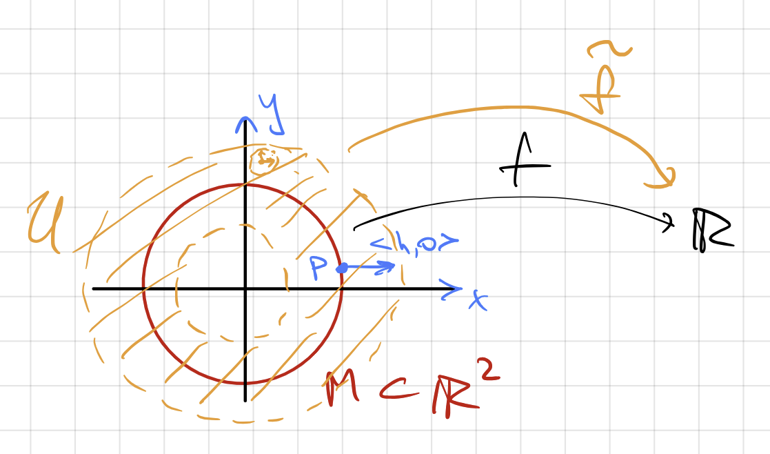
Recall local coordinates: For any $p\in M$ there is a set $V\ni p$ open in ${ℝ}^n$ and $U$ open in $M$ with

$$\phi :V\to U$$

a parametrization (diffeomorphism to its image). The ${ℝ}^n$-coordinates of images of the inverse ${\phi }^{-1}$ give local coordinates on $U$.

Critical and non-degenerate, from a manifold

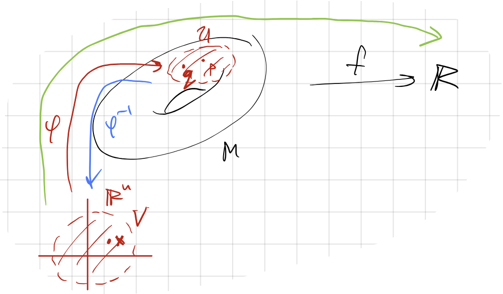
Let $f:M\to ℝ$ be a smooth function on a smooth $n$-manifold in ${ℝ}^d$, and $\phi :V\to U$ a parametrization of the open neighborhood $U$ of $p$. So $f\circ \phi :V\to ℝ$ for $V\subset {ℝ}^n$.

Choose any $q\in U$. Set $x={\phi }^{-1}(q)$.

We say $q$ or $x$ is regular when $\nabla (f\circ \phi )(x)\ne \overrightarrow{0}$ and critical when $\nabla (f\circ \phi )(x)=\overrightarrow{0}$.

We say $q$ or $x$ is non-degenerate when $[H_x(f\circ \phi )]$ is a non-singular matrix (and degenerate otherwise).

Notice that this definition of regularity appears to depend on the parametrization $\phi$. But in fact, the definition is independent of the choice of $\phi$:

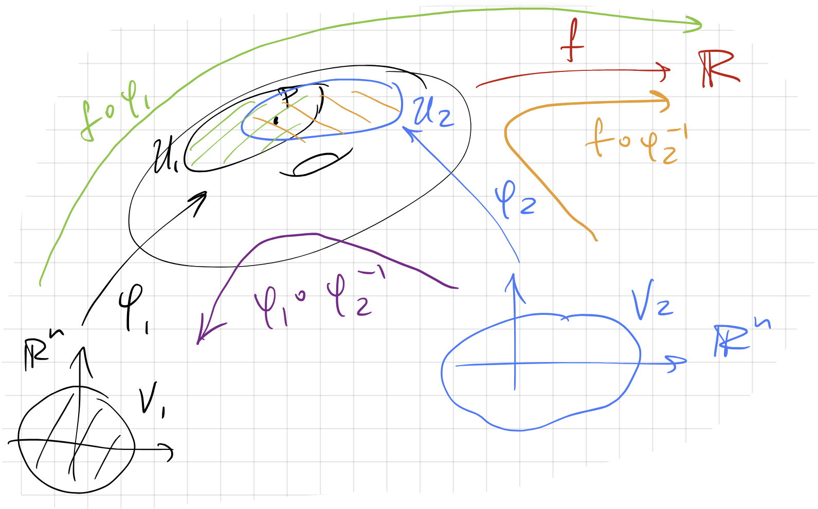
Proposition - Regularity is independent of parametrization

Suppose we are given two parametrizations ${\phi }_1$ and ${\phi }_2$ of a coordinate patch $U\subset M$.

Take an arbitrary $q\in U$ and assume it is regular according to ${\phi }_1$.

We show it must be regular according to ${\phi }_2$.

This will complete the proof because if it is critical according to ${\phi }_1$, and not critical according to ${\phi }_2$, then it is regular according to ${\phi }_2$, and the same argument can be run after switching ${\phi }_1\leftrightarrow {\phi }_2$.

---

Define the ‘transition map’ $\psi ={\phi }_1^{-1}\circ {\phi }_2$.

This $\psi$ is a map $V_1\to V_2$ where ${\phi }_1:V_1\to U$ and ${\phi }_2:V_2\to U$ for $V_i\subset {ℝ}^n$ open balls.

Notice that $(f\circ {\phi }_2)=(f\circ {\phi }_1)\circ \psi$.

---

Apply chain rule:

$$\nabla (f\circ {\phi }_2)=\nabla (f\circ {\phi }_1\circ \psi )=\nabla (f\circ {\phi }_1)\circ [d\psi ]$$

Here $[d\psi ]$ is the Jacobi matrix of $\psi$.

---

Argue that $[d\psi ]$ is invertible:

We have that $[d{\phi }_1]$ and $[d{\phi }_2]$ are both isomorphisms from ${ℝ}^n$ to the tangent space of $M$ at $q$.

Then $[d\psi ]$ is the composition of $[d{\phi }_2]$ with the inverse of $[d{\phi }_1]$ restricted to the tangent space of $M$ at $q$. (Prior to restriction $[d{\phi }_1]$ is not even a square matrix.)

Therefore $[d\psi ]$ is invertible.

Therefore, at any point:

$$\nabla (f\circ {\phi }_2)=0⟺\nabla (f\circ {\phi }_1\circ \psi )=0$$

So a point is regular for ${\phi }_1$ if and only if it is regular for ${\phi }_2$.

Why define regularity using parametrizations?

Since the choice of parametrization has no effect on the classification of points as regular or critical, one may wonder why the parametrization is needed at all.

But the concept of regularity does involve the manifold’s embedding, and not just the values of $f$ in the ambient space around the manifold.

A point $q\in M$ is regular for $f$ when there is some first-order infinitesimal deviation of $q$ within $M$ which causes a first-order deviation in $f$. When $q$ is critical, the induced change in $f$ is second order at most.

For example, given a smooth function $f:{ℝ}^n\to ℝ$, a level surface $M$ is (frequently) an $(n-1)$-manifold every point of which is regular for $f:{ℝ}^n\to ℝ$, but no point of which is regular for $f{|}_M:M\to ℝ$.

Tangent space $T_{p}M$

Given a manifold $M\subset {ℝ}^d$, we define the tangent space to $M$ at $p\in M$, written $T_{p}M$, as the image of $[d_p\phi ]$ in ${ℝ}^d$ for $\phi$ any parametrization of a neighborhood of $p$.

Comparing gradient functions

Notice:

• $\nabla \tilde{f}$ is a map from ${ℝ}^d$, and has $d$ coordinates
• $\nabla (f\circ \phi )$ is a map from ${ℝ}^n$, and has $n$ coordinates, one for each dimension of $M$

In general: ${\nabla }_p(f\circ \phi )$ is the restriction of ${\nabla }_p\tilde{f}$ to $T_{p}M$ using columns of $[d\phi ]$ as a basis.

(Supposing $M\subset {ℝ}^d$ and $\tilde{f}$ an extension of $f:M\to ℝ$ to $U$ with $M\subset U\subset {ℝ}^d$.)

---

Morse Lemma

Suppose $q$ is a non-degenerate critical point of index $i$ of a smooth function $f:M\to ℝ$.

Then:

$$f\circ \phi =x_1^2+\cdots +x_{n-i}^2-x_{n-i+1}-\cdots -x_n^2$$

for some parametrization $\phi$ whose local coordinates are $x_1,\dots ,x_n$.

Morse functions

A Morse function $f:M\to ℝ$ is a smooth function from a manifold $M\subset {ℝ}^d$ to $ℝ$ which satisfies:

1. All critical points of $f$ are non-degenerate.
2. The values of $f$ at its critical points are all distinct.

Morse functions are dense

Morse functions are dense in the space of smooth functions.

There is a small perturbation of any smooth function that is a Morse function.

06 Illustration

Height function

Suppose $\tilde{f}:{ℝ}^3\to ℝ$ by $\tilde{f}(x,y,z)=z$.

Then $\nabla \tilde{f}=(\mathrm{0,0,1})$. Since $\nabla (f\circ \phi )$ is the restriction of $\nabla \tilde{f}$ to $T_{p}M$, we see that $p$ is critical for $f$ precisely when $T_{p}M$ is normal to $(\mathrm{0,0,1})$.

In other words: critical points of $f$ are points where the tangent space to $M$ is a horizontal plane.

This reasoning generalizes to higher dimensions ${ℝ}^d$ where one dimension is chosen as ‘vertical’, and horizontal planes become hypersurfaces normal to the vertical unit vector.

07 Theory - Morse functions and topology

Given a Morse function $f:M\to ℝ$ for a manifold $M$, define:

• $M_C=f^{-1}(C)$ the level set at $C$
• $M_{\le C}=f^{-1}((-\infty ,C])$ the sublevel set under $C$

By continuously increasing the value of $C$ (starting at $-\infty$), we find that the topology of $M_{\le C}$ changes exactly when $C$ passes a critical point of $f$.

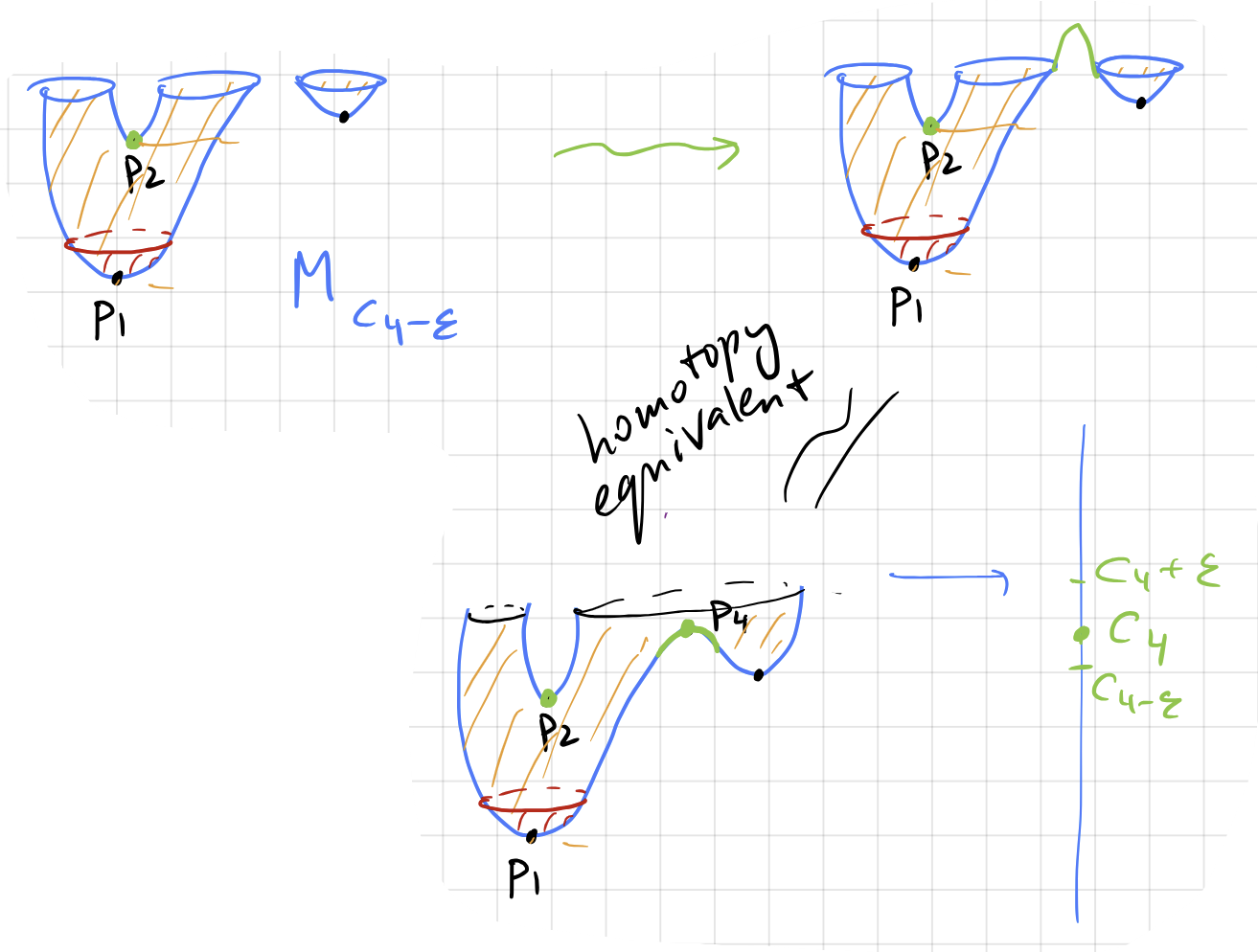
Sublevel set builds topology

Up to homotopy equivalence, as $C$ passes through a critical point of index $k$, the sublevel set changes by the attachment of a $k$-ball along its boundary.

For example:

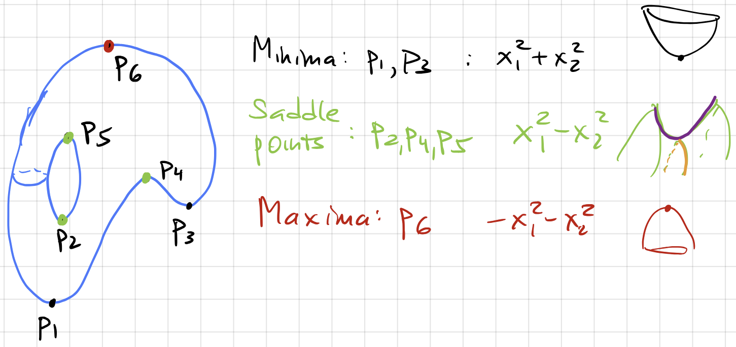
• Pass a point of index $2$ $⇝$ glue on a disk, a lid opening downwards
• Pass a point of index $1$ $⇝$ glue on an arc (up to homotopy)
• Pass a point of index $0$ $⇝$ create a new disk, a basket opening upwards

08 Illustration

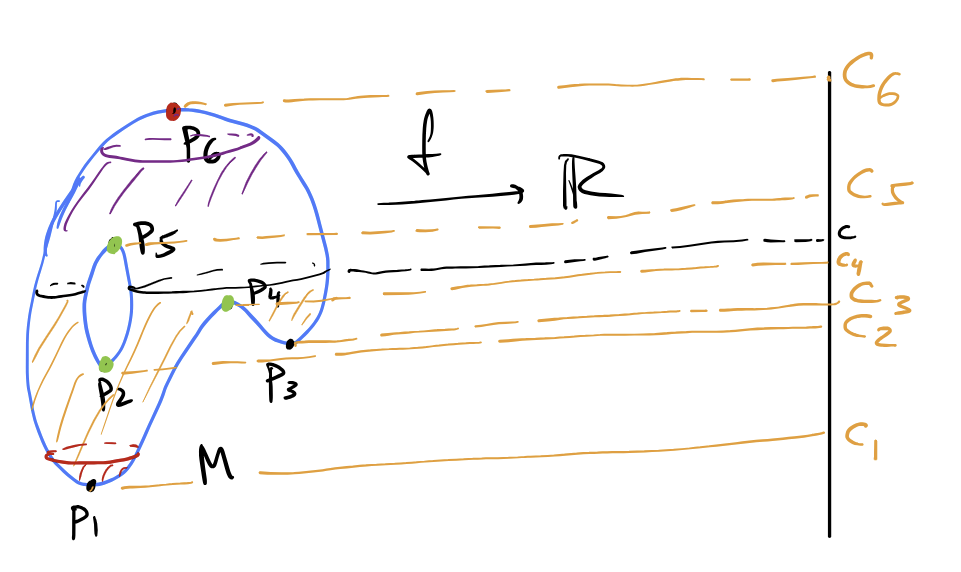
Height function on a torus

Suppose $f:{ℝ}^3\to ℝ$ is the height function $f(x,y,z)=z$, and $M$ is topologically a torus, though not geometrically.

As $C$ passes through $f(P_1)$, a small disk is created in $M_{\le C}$.

Passing through $f(P_2)$ is (up to homotopy) equivalent to adding a handle to the basket below $C_2$:

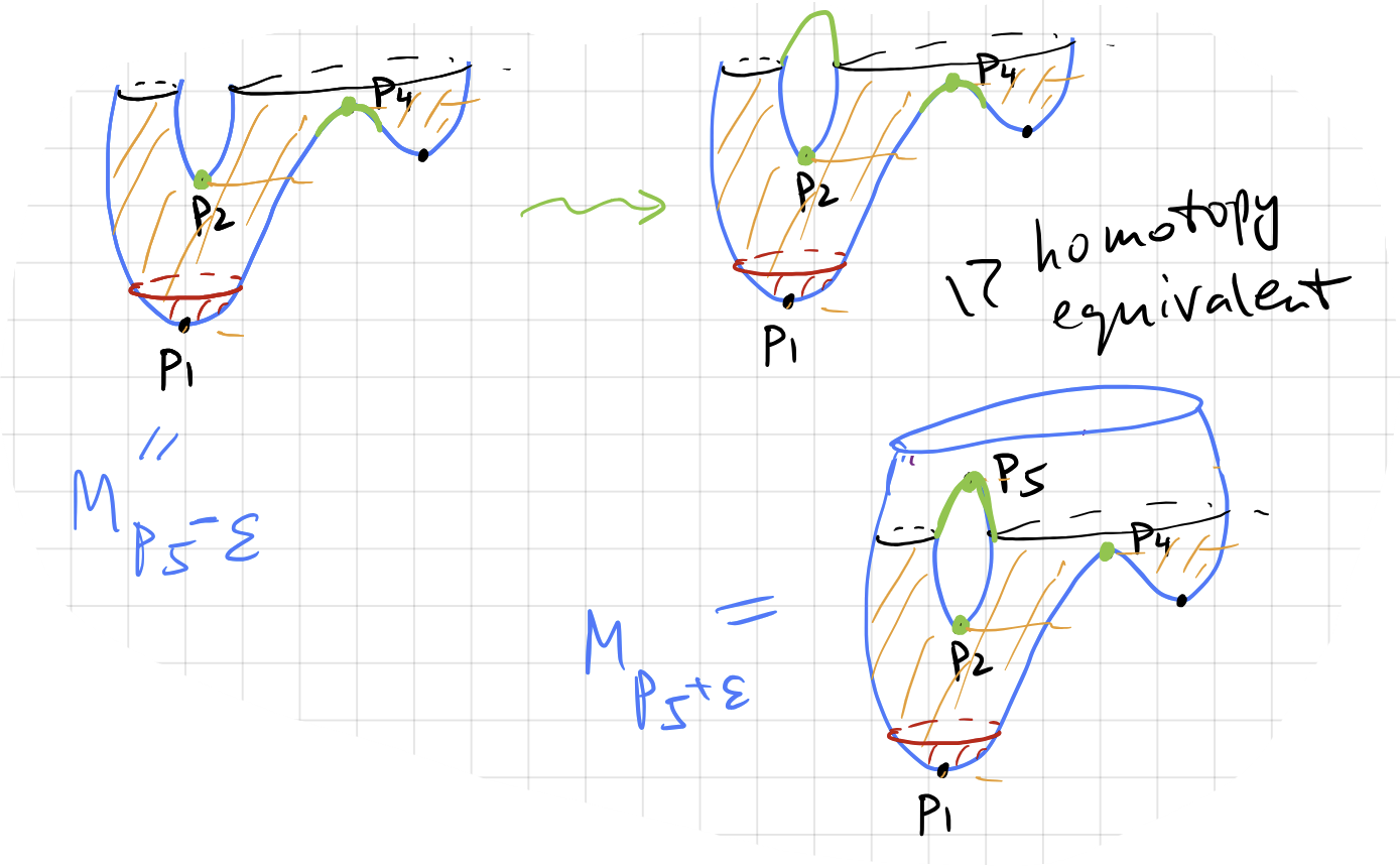
Passing through $f(P_3)$ adds a new basket, and passing through $f(P_4)$ adds a handle connecting the basket:

Passing through $f(P_5)$ adds a handle creating a loop:

Structures from point-cloud data

09 Theory - Gromov-Hausdorff distance

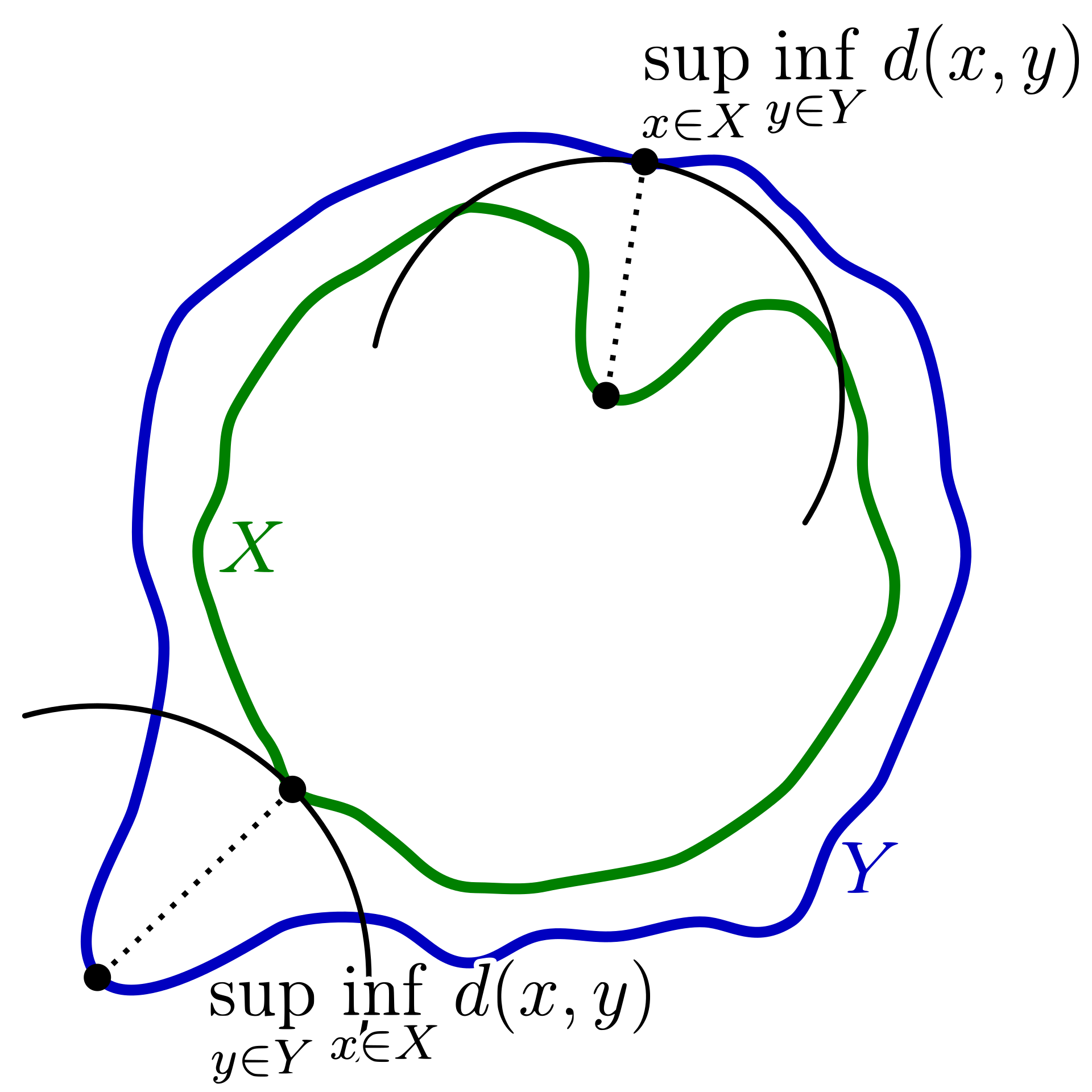
Hausdorff distance

Suppose $A$ and $B$ are subsets of a metric space $(X,d)$.

The Hausdorff distance is:

$$d_H(A,B)=\max (\underset{x\in A}{\sup }d(x,B),\underset{y\in B}{\sup }d(A,y))$$

Here:

• $d(x,B)=\underset{y\in B}{\inf }d(x,y)$ $$ smallest distance $x$ to $B$
• $d(A,y)=\underset{x\in A}{\inf }d(x,y)$ $$ smallest distance $y$ to $A$

Therefore:

• $\underset{x\in A}{\sup }d(x,B)$ $$ within $A$, how far away can you get from $B$?
• $\underset{y\in B}{\sup }d(A,y)$ $$ within $B$, how far away can you get from $A$?

Gromov-Hausdorff distance

Suppose $A$ and $B$ are compact metric spaces and $(X,d)$ is some fixed compact metric space.

The Gromov-Hausdorff (GH) distance is:

$$d_{GH}(A,B)=\underset{f,g}{\inf }{d}_H(f(A),g(b))$$

where $f$, $g$ are isometric embeddings of $A$, $B$ into $X$.

Notice that this definition is relative to $(X,d)$.

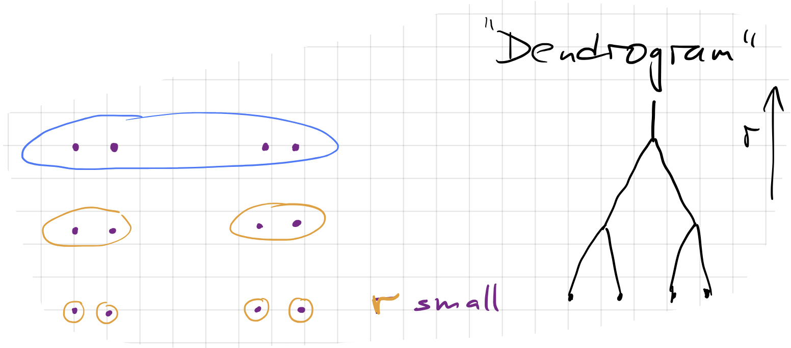
10 Theory - Dendrogram

Persistent homology describes the clustering of point-cloud data.

The GH distance frequently serves as a pure math benchmark. Given finite sets of points $P,Q\subset {ℝ}^d$, the distance $d_{GH}(P,Q)$ is a measure of similarity of the shape of the point clouds $P$ and $Q$.

The GH distance cannot be computed efficiently (if at all), so other measures of similarity for point clouds are useful.

Desiderata for measures of point-cloud similarity:

• Quantifies topological and geometric features
• Distinguishes features from noise
• Is computable
• Recognizes when features are close in the GH metric

---

Suppose we have a finite set of points $P\subset X$ for a metric space $(X,d)$.

Fix $r\in {ℝ}_{\ge 0}$. Define a relation $x_1{\sim }_r{x}_2$ when $d(x_1,x_2)\le r$.

Let ${\simeq }_r$ be the transitive closure of ${\sim }_r$. This is an equivalence relation (generated by ${\sim }_r$) which partitions $P$ into equivalence classes. Members of each equivalence class can be obtained from one another by a sequence of “hops” between points no more than $r$ apart.

Draw a tree diagram with a junction at each $r$ where distinct clusters are joined:

11 Theory - Filtrations

Filtered simplicial complex

A filtered simplicial complex is a complex $𝒦$ with a collection:

$$\varnothing \subset {𝒦}_{a_1}\subset {𝒦}_{a_2}\subset \cdots \subset {𝒦}_{a_n}=𝒦$$

where each ${𝒦}_{a_i}$ is a simplicial complex which is a subcomplex of ${𝒦}_{a_{i+1}}$.

(The vertices and simplices of a subcomplex must be vertices and simplices in the supercomplex.)

Filtered space

A filtered topological space is a collection $X_t$ of spaces indexed by $t\in [0,\infty ]$ with continuous maps:

$$f_{s,t}:X_s\to X_t\text{each }s\le t$$

and these maps satisfy a transitivity compatibility:

$$X_r\stackrel{f_{r,s}}{⟶}{X}_s\stackrel{f_{s,t}}{⟶}{X}_t{f}_{r,t}=f_{s,t}\circ f_{r,s}$$

It is sometimes convenient, if a little ungainly, to consider a filtered simplicial complex as a filtered space where ${𝒦}_s$ is a simplicial subcomplex of ${𝒦}_t$ whenever $s\le t$. Such a filtered space changes only at discrete values of $t$.

12 Illustration

Čech complex as filtered complex

Let $𝒫=\{p_1,\dots ,p_n\}$ be a finite set of points in a metric space $(X,d)$.

Recall that the Čech complex of $𝒫$, written ${𝒫}_r$ for $r\in [0,\infty )$, is the nerve complex of the collection of open balls $\{B_r(p_i)\}$.

In other words, ${𝒫}_r$ is the complex with vertices the points of $𝒫$, and $k$-simplices the subsets $\sigma \subset 𝒫$ with $k+1$ points whose $r$-balls have nonempty mutual intersection.

This is a filtered complex because $B_r(p_i)\subset B_s(p_i)$ whenever $r\le s$. Once in, always in, for a simplex.

13 Theory - Vietoris-Rips complex

Vietoris-Rips complex

Let $𝒫=\{p_1,\dots ,p_n\}$ be a finite set of points in a metric space $(X,d)$.

The Vietoris-Rips complex $\mathrm{VR}(𝒫,r)$ is the complex whose vertices are the points $𝒫$, and whose $k$-simplices are those subsets $\sigma \subset 𝒫$ with $k+1$ points all of which are pairwise less than $2r$ apart:

$$\begin{array}{cc}& [p_{i_0},\dots ,p_{i_k}]\\ & k\text{-simplex}\in 𝒫\end{array}⟷\begin{array}{cc}& d(p_j,p_{\ell })<2r\\ & \forall j,\ell \in \{i_0,\dots ,i_k\}\end{array}$$

The VR complex is a filtered space (filtered complex) because:

$$\mathrm{VR}(𝒫,r)\subset \mathrm{VR}(𝒫,s)\subset \mathrm{VR}(𝒫,t)\text{when}r\le s\le t$$

Notice that the VR complex and the Čech complex include the same 1-simplices: a simplex $\sigma =[p_i,p_j]$ is in the VR complex if $d(p_i,p_j)<2r$, and in the Čech complex if $B_r(p_i)\cap B_r(p_j)\ne \varnothing$. These conditions are equivalent, at least in ${ℝ}^d$.

Pairwise vs. mutual intersection

• The VR complex includes simplices for points which pairwise intersect.
• The Čech complex includes simplices for points which mutually intersect.

For example:

The three blue circles all intersect pairwise, so $[p_1,p_2,p_3]$ is in the VR complex, but they don’t mutually intersect so this simplex is not in the Čech complex.

On the other hand, the four green circles do not intersect pairwise. The VR complex and the Čech complex are the same in this case.

VR complex computability

Since the VR complex depends only on the data of pairwise distances between points, it is very easy to compute.

---

Čech and VR containments

For any point cloud $𝒫\subset {ℝ}^d$, we have:

1. $\check{\mathrm{C}}\mathrm{e}\mathrm{c}\mathrm{h}(𝒫,r)\subset \mathrm{VR}(𝒫,r)$ $$ inclusion as subcomplex
2. $\mathrm{VR}(𝒫,r)\subset \check{\mathrm{C}}\mathrm{e}\mathrm{c}\mathrm{h}(𝒫,2r)$ $$ inclusion as subcomplex

The first is true because any mutual intersection implies the pairwise intersections.

The second is true because any pairwise intersection of $B_r$ balls implies that the $B_{2r}$ balls extend to cover other centers. So the centers of all points are in the $2r$-balls of each of the others, thus the centers are in the mutual intersection.

14 Theory - Persistent homology, barcodes

Persistent homology

Let ${𝒦}_t$ be a filtered simplicial complex.

Fix $k\in \mathbb{N}$. For any $t\in [0,\infty )$, define:

$$V_k^t=H_k({𝒦}_t;ℝ)$$

Whenever $s\le t$ there is a map ${𝒦}_s\to {𝒦}_t$ and this induces linear maps on homology:

$$L_k^{s,t}:V_k^s\to V_k^t$$

These satisfy $L_k^{r,t}=L_k^{s,t}\circ L_k^{r,s}$.

The persistent homology of ${𝒦}_t$ is the collection of vector spaces $V_k^t$ and linear maps $L_k^{s,t}$.

Persistent homology is defined for any filtered simplicial complex. For example, we can take persistent homology of the Čech complex or of the Vietoris-Rips complex.

Persistent VR homology - Structure Theorem

Let $V_k^r=H_k(\mathrm{VR}(𝒫,r))$ for $r\in [0,\infty )$ be the persistent homology of the VR complex of a point cloud $𝒫$.

Fix $k\in \mathbb{N}$. Then ${\{V_k^r\}}_{r\in {ℝ}^{>0}}$ has a canonical decomposition as a direct sum of persistence intervals:

$${\{V_k^r\}}_{r\in {ℝ}^{>0}}\stackrel{\sim }{⟶}\underset{i}{⨁}\mathrm{P}(a_i,b_i)$$

Persistence interval

For any $a<b$ with $a\in [0,\infty )$ and $b\in [0,\infty ]$, define:

$$\mathrm{P}(a,b{)}_r=\{\begin{array}{cc}ℝ& r\in [a,b)\\ \{0\}& r\notin [a,b)\end{array}$$

with (linear) filtration maps $L^{r,s}:\mathrm{P}{(a,b)}_r\to \mathrm{P}{(a,b)}_s$ given by $L^{r,s}={\mathrm{Id}}_{ℝ}$ when $r,s\in [a,b)$.

15 Illustration

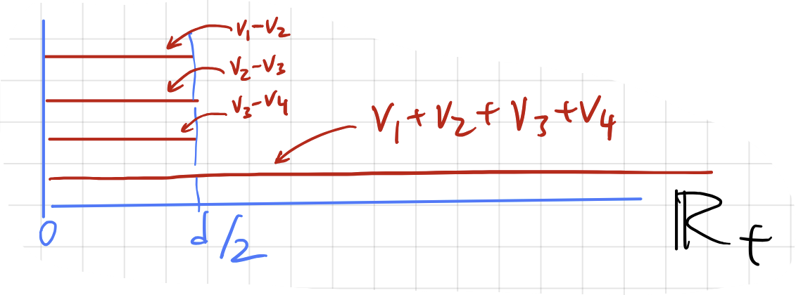
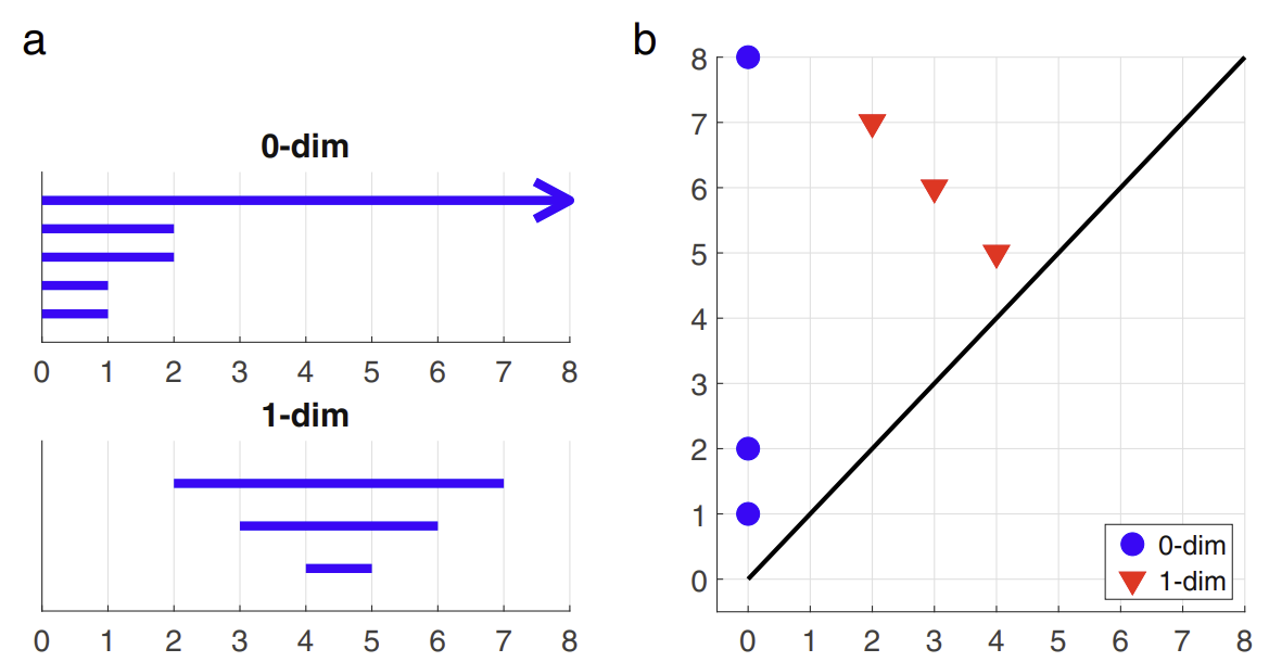
Barcode diagram:

• Each $\mathrm{P}(a_i,b_i)$ receives a horizontal bar starting at $a_i$, ending at $b_i$.
• Bar colored according to degree $k$ in $H_k(\mathrm{VR}(𝒫,r))$

Persistence diagram:

• Each $\mathrm{P}(a_i,b_i)$ receives a dot placed at $(a_i,b_i)$
• Horizontal ‘birth’ axis, vertical ‘death’ axis
• Dots colored according to degree $k$ in $H_k(\mathrm{VR}(𝒫,r))$

Point cloud: square

Basis:

Decomposition:

$$H_0(\mathrm{VR}(𝒫),r)\stackrel{\sim }{⟶}{\oplus ︎}^3\mathrm{P}(0,d/2)\oplus ︎\mathrm{P}(0,\infty )$$

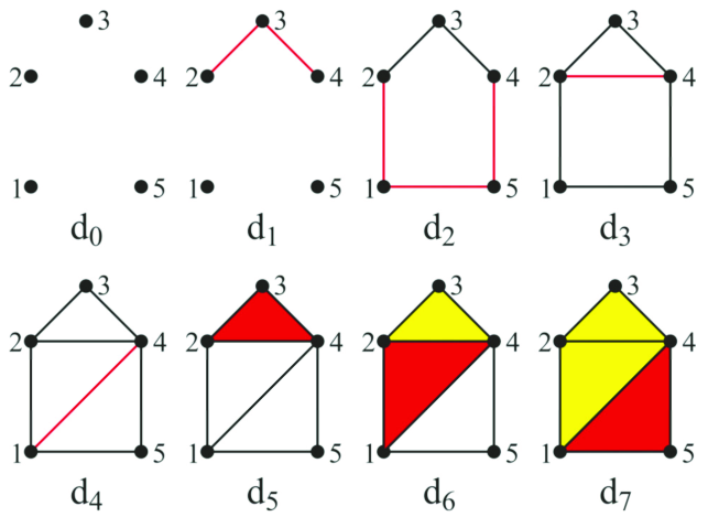
Filtered complex

Abstract filtration:

Barcode and persistence diagram:

16 Theory - Barcode basis

We would like to understand the direct sum decompositions like the one in the example of the point cloud square:

$$H_0(\mathrm{VR}(𝒫),r)\stackrel{\sim }{⟶}{\oplus ︎}^3\mathrm{P}(0,d/2)\oplus ︎\mathrm{P}(0,\infty )$$

Understanding such a decomposition amounts to determining a basis of homology classes that have lifespans described by the persistence intervals.

We have:

$$H_0(\mathrm{VR}(𝒫,r_2))\cong \frac{\ker ({\partial }_0)}{\mathrm{im}({\partial }_1)}\text{⨠}\text{⨠}\frac{{ℝ}^2}{ℝ}$$

A basis for $H_0$ is the equivalence class of all vectors in ${ℝ}^2$ which are not in the span $⟨v_2-v_1⟩$. For example, $v_1$ or $v_2$ or $v_1+v_2$.

Barcode diagram for $H_0$:

---

Now consider $H_1$. Cycles in $H_1$ are generated by 1-simplices which are sets of two points that are $\le 2r$ apart.

Consider again the square point cloud:

For $r<\frac{d}{2}$, we have $\mathrm{VR}(𝒫,r)=\text{4 discrete points}$.

For $r=\frac{d}{2}+\epsilon$, we have $\mathrm{VR}(𝒫,r)=\text{square}\simeq {𝕊}^1$.

For $r=\frac{d}{2}\sqrt{2}$, we have 4 additional 2-simplices (all combinations of 3 points).

The square will the boundary of the difference of two of the 2-simplices (complementary triangles), so the homology class of the square vanishes when $r$ reaches $\frac{d}{2}\sqrt{2}$.

Barcode diagram for $H_1$:

---

Thus:

$$\begin{array}{cc}{H}_0& \cong \mathrm{P}{(\mathrm{0,1})}^{\oplus ︎3}\oplus ︎\mathrm{P}(0,\infty )\\ & \\ H_1& \cong \mathrm{P}(\frac{d}{2},\frac{d}{2}\sqrt{2})\end{array}$$