TDA Notes - Unit 04

Stability

01 Theory - Bottleneck distance

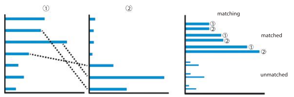
The bottleneck distance is a metric on barcode diagrams. The bars in one barcode are matched against the bars in the other. The distance between barcodes is the worst discrepancy between bars in the optimal matching.

Suppose we are given two barcode diagrams. These are two finite collections of intervals:

$$\begin{array}{c}𝕀=\{I_a{\}}_{a\in A},𝕁=\{J_b{\}}_{b\in B}(A,B\text{ finite})\\ \\ I_a=[x_a,y_a),J_b=[x_b,y_b)\end{array}$$

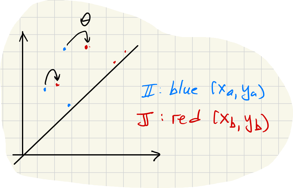
Now define the $d_{\infty }$-distance between two intervals by:

$$d_{\infty }(I_a,J_b)=\max (|x_b-x_a|,|y_b-y_a|)$$

Also, define:

$$\lambda (I_a)=d_{\infty }(I_a,\varnothing )=\frac{|y_a-x_a|}{2}$$

This is the $d_{\infty }$-distance to the nearest point-interval $(x,x)$.

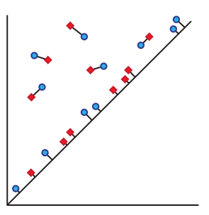
Now, suppose we are given subsets $A^{\prime }\subset A$ and $B^{\prime }\subset B$ along with a choice of bijection $\theta :A^{\prime }\to B^{\prime }$. Define the penalty of $\theta$ to be:

$$P_{\infty ;A^{\prime },B^{\prime },\theta }=\max \left(\begin{array}{cc}& {\max }_{a\in A^{\prime }}{d}_{\infty }(I_a,J_{\theta (a)})\\ & {\max }_{a\in A\backslash A^{\prime }}\lambda (I_a)\\ & {\max }_{b\in B\backslash B^{\prime }}\lambda (J_b)\end{array}\right)$$

Bottleneck distance

The bottleneck distance from $𝕀$ to $𝕁$ is:

$$d_{\infty }(𝕀,𝕁)=\underset{\begin{array}{c}{A}^{\prime }\subset A\\ B^{\prime }\subset B\\ \theta :A^{\prime }\to B^{\prime }\end{array}}{\min }{P}_{\infty ;A^{\prime },B^{\prime },\theta }$$

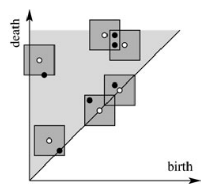
Bars far from the diagonal are matched to the closest bars (using the ${\ell }_{\infty }$-norm whose unit balls are squares). Bars near the diagonal can be matched to the closest diagonal point. The distance to the closest point on the diagonal is $\lambda (I_a)$.

Stability Theorem: Bottleneck Distance

Let $𝒫$ and $𝒬$ be two finite metric spaces. Fix $k\in {\mathbb{Z}}_{\ge 0}$. Let $B_{𝒫}$ be the barcode diagram for $H_k(\mathrm{V}\mathrm{R}(𝒫,\mathrm{r}))$ and let $B_{𝒬}$ be the barcode diagram for $H_k(\mathrm{VR}(𝒬,r))$. Then:

$$d_{\infty }(B_{𝒫},B_{𝒬})\le d_{GH}(𝒫,𝒬)$$

This theorem is a kind of “stability” result regarding barcode diagrams, since it says that when two data sets $𝒫$ and $𝒬$ are close together (measured using the ideal, if not computable, metric $d_{GH}$), then the barcode diagrams are also close together. Barcode diagrams cannot jump apart without the data sets jumping apart.

For example, if $𝒫$ is a “noisy” version of $𝒬$, then we expect $d_{GH}(𝒫,𝒬)$ to be small, and therefore the barcode diagrams should be close. Conversely, if barcode diagrams are far, the data sets differ by “more than noise.”

02 Theory - Wasserstein metrics

The Wasserstein metrics generalize the bottleneck metric. Instead of taking the worst discrepancy between two bars in the best matching, it uses a $p$-sum of the discrepancies of all bars in the best matching.

First define the $p$-penalty for a partial matching $\theta :A^{\prime }\to B^{\prime }$ as follows:

$$P_{p;A^{\prime },B^{\prime },\theta }={(\sum _{a\in A^{\prime }}{d}_{\infty }{(I_a,J_{\theta (a)})}^p+\sum _{a\in A\backslash A^{\prime }}\lambda {(I_a)}^p+\sum _{b\in B\backslash B^{\prime }}\lambda {(J_b)}^p)}^{1/p}$$

Then we minimize the penalty (find the best matching):

$$d_p(𝕀,𝕁)=\underset{\begin{array}{c}{A}^{\prime }\subset A\\ B^{\prime }\subset B\\ \theta :A^{\prime }\to B^{\prime }\end{array}}{\min }{P}_{p;A^{\prime },B^{\prime },\theta }$$

Remark

We can recast the $p$-penalty in a more uniform symbolism by supplementing $A$ or $B$ with empty bars so that each has the same number of “bars,” and recalling the convention that $d_{\infty }(I_a,\varnothing )=\lambda (I_a)$. Then we have:

$$d_p(𝕀,𝕁)=\underset{\theta :A\to B}{\min }{\left(\sum _{a\in A}{(||a-\theta (a)|{|}_{\infty })}^p\right)}^{1/p}$$

Multi-dimensional persistent homology

03 Theory - Several parameters

Thus far the persistent homology we have considered is derived from filtered spaces/complexes with a single filtration parameter $r$:

$$\mathrm{VR}(𝒫,r),f^{-1}((-\infty ,r))$$

It is possible to combine two types of filtration in a single structure having inclusion maps of each type.

Unfortunately there is no “structure theorem” for persistent homology with more than one parameter. This is basically because the structure theorem proof in one parameter involves homology with $ℝ[x]$ coefficients, while with $n$ parameters it involves homology with $ℝ[x_1,\dots ,x_n]$ coefficients.

04 Illustration

Filtering also by density

Let us add a density filtration to $\mathrm{VR}(𝒫,r)$. Fix $k\in {\mathbb{Z}}_{\ge 0}$ and define $\rho :𝒫\to ℝ$ by:

$$\rho (x_i)=\frac{1}{d_k(x_i)},d_k(x_i)=\text{distance to }{k}^{th}\text{ nearest neighbor}$$

Now the points in $𝒫$, and the $\mathrm{VR}$-complex itself, can be filtered by a density minimum:

$$\mathrm{VR}(𝒫,r,s)=\mathrm{VR}(\{x\in 𝒫|\rho (x)\ge s\},r)$$

This bi-filtered complex determines a 2-parameter persistence module:

$$H_k(\mathrm{VR}(𝒫,r,s))$$

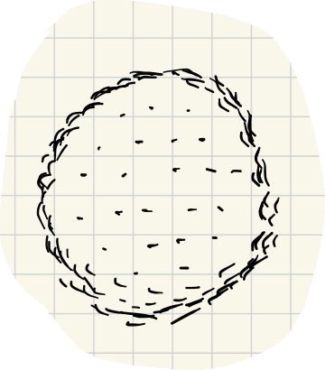
For large $s$, only points very close to $k$ distinct neighbors are included. As $s$ decreases, more points are brought in.

With data like this, the $s$ filtration (for middling $s$ values) removes points inside the disk because they are too sparse.

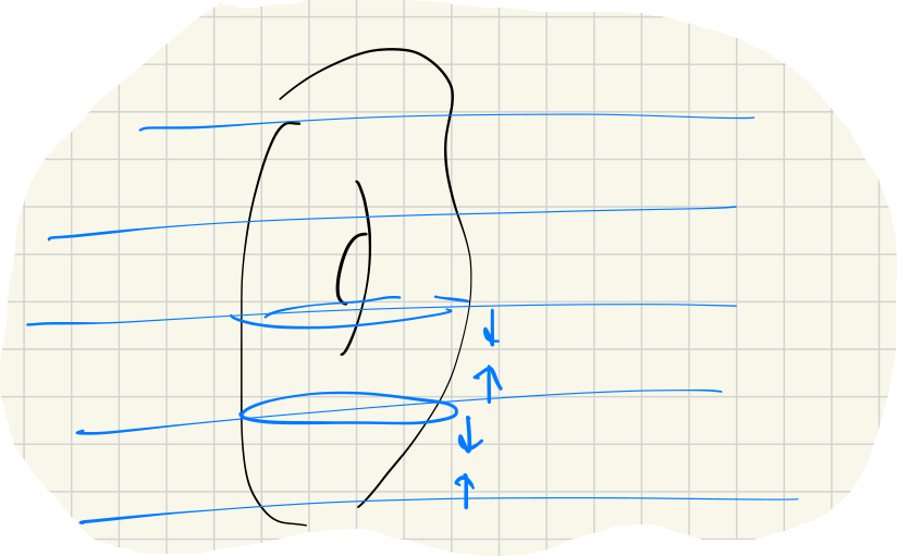
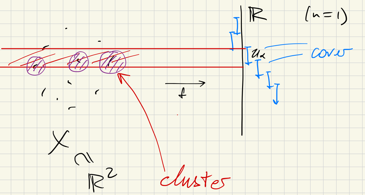
Filtering also by distance to a subspace

Suppose $\iota :{ℝ}^k\hookrightarrow {ℝ}^n$ is an embedded $k$-dimensional subspace of the background space ${ℝ}^n$ that contains the data:$𝒫\subset {ℝ}^n$.

Let $f_{\iota }:𝒫\to ℝ$ measure the distance from data points to the image of $\iota$.

Define ${𝒫}_R=f^{-1}((-\infty ,R))$. This gives a filtration in terms of the parameter $R$. This filtration could be useful if the complete data set $𝒫$ is too big to process all at once. The filtration allows one to process the data in layers.

These filtrations determine inclusions of $\mathrm{VR}$ complexes. For fixed $R$ and $r<s$, we have:

$$\mathrm{VR}({𝒫}_R,r)\subset \mathrm{VR}({𝒫}_R,s)$$

Upon applying homology, for $k\in {\mathbb{Z}}_{\ge 0}$, we have:

$$H_k(\mathrm{VR}({𝒫}_R,r))\stackrel{L_{r,s}^R}{⟶}{H}_K(\mathrm{VR}({𝒫}_R,s)))$$

And for fixed $r$ and $R<S$, we have:

$$\mathrm{VR}({𝒫}_R,r)\subset \mathrm{VR}({𝒫}_S,r)$$

Upon applying homology, we have:

$$\mathrm{VR}({𝒫}_R,r)\stackrel{L_r^{R,S}}{⟶}\mathrm{VR}({𝒫}_R,s)$$

Finally, these induced maps should commute with each other:

$$L_s^{R,S}\circ L_{r,s}^R=L_{r,s}^S\circ L_r^{R,S}$$

05 Theory - Zig-zag persistent homology

Filtrations can be modified in another way by adding intermediate linking sets. Instead of the usual filtered space like this:

$${𝒦}_{r_1}\subset {𝒦}_{r_2}\subset {𝒦}_{r_3}\subset \cdots$$

We have a “zig-zag” filtered space like this:

$${𝒦}_1\hookleftarrow {𝒦}_{\mathrm{1,2}}\hookrightarrow {𝒦}_2\hookrightarrow {𝒦}_{\mathrm{2,3}}\hookleftarrow {𝒦}_3\hookrightarrow \cdots$$

In general, each arrow is allowed to go either direction. The induced map on homology will follow the same pattern.

06 Illustration

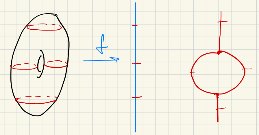
Morse layers

An application of zig-zag filtration arises by dividing the entire space into small layers for which the homology is easier to compute. For example, with a Morse function $f:𝒦\to {ℝ}_{\ge 0}$, we have this zig-zag filtration:

$$f^{-1}(0)\hookrightarrow f^{-1}([\mathrm{0,1}])\hookleftarrow f^{-1}(1)\hookrightarrow f^{-1}([\mathrm{1,2}])\hookleftarrow f^{-1}(2)\hookrightarrow \cdots$$

Repeated samples

Suppose some data is sampled repeatedly and data sets are generated in a sequence:

$$X_1,X_2,X_3,X_4,\dots$$

Then we can form a zig-zag filtration by:

$$X_1\hookrightarrow X_1\cup X_2\hookleftarrow X_2\hookrightarrow X_2\cup X_3\hookleftarrow X_3\hookrightarrow X_3\cup X_4\hookleftarrow \cdots$$

Mapper algorithm

07 Theory - Clustering and Reeb graph

The mapper algorithm was introduced by Singh-Mémoli-Carlsson in 2007.

Recall the dendrogram (clustering) algorithm:

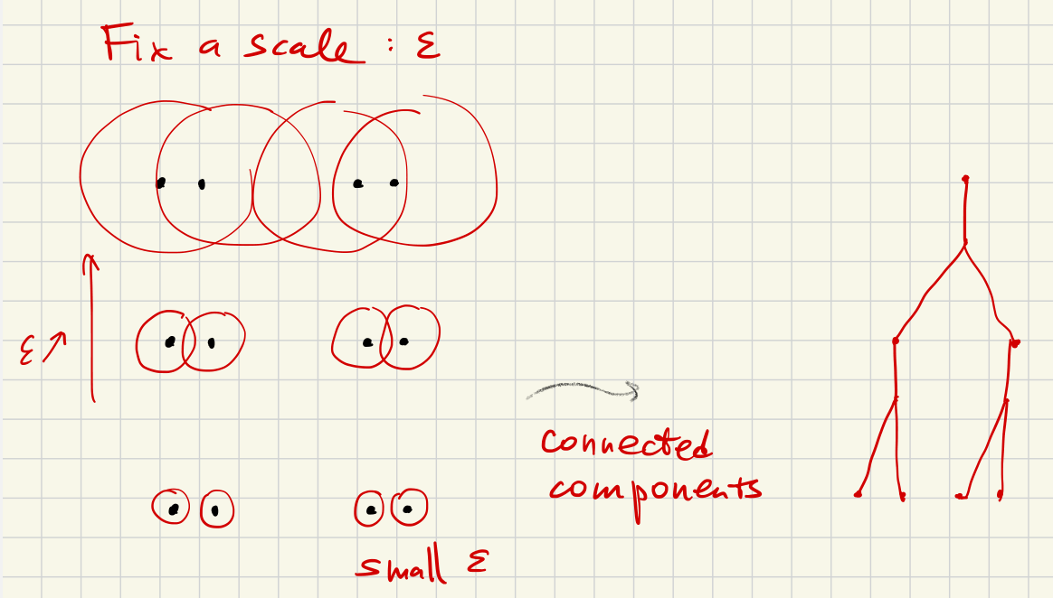
Given a fixed $\epsilon >0$, two points $x,y$ are considered equivalent if there is a sequence of points

$$x=x_0,x_1,x_2,\dots ,x_k=y$$

and the distance between successive points is much less than $\epsilon$.

Now consider connected components (“clusters”) for each fixed $\epsilon$. The clustering algorithm computes this and the calculation is essential the same as persistent homology $H_k$ for $k=0$.

Reeb graph

Given a Morse function $f:M\to ℝ$ on a manifold $M$, the Reeb graph is formed by the equivalence relation:

Two points $x,y\in M$ are equivalent if:

• $f(x)=f(y)$ AND
• $x,y$ are in the same connected component of $f^{-1}(f(x))$

08 - Mapper algorithm

Let us be given:

• A finite metric space $(X,d)$
  • I.e. a finite collection of points $\{x_1,x_2,\dots ,x_k\}$ with distances between them; usually $X\subset {ℝ}^n$
• A “filter function” $f:X\to {ℝ}^n$
• A finite cover $𝒞={\{C_{\alpha }\}}_{\alpha \in A}$ of $f(X)$ in ${ℝ}^n$
  • Typically a collection of boxes in ${ℝ}^n$

Proceed as follows:

(1) Consider the clustering of each $f^{-1}(U_{\alpha })$:

• Choose $\epsilon >0$ and consider clusters at this scale $\epsilon$.
• Write $C_{\alpha ,i}$ for the clusters, so $f^{-1}(U_{\alpha })={⨆}_i{C}_{\alpha ,i}$

(2) Form a discrete version of the Reeb graph:

• Vertices: clusters $C_{\alpha ,i}$
• Edges: when $C_{\alpha ,i}$ and $C_{\beta ,j}$ overlap
• Color the vertices according to values of $f$ (on average):

09 Illustration

Simple cover

Suppose $f:X\to ℝ$ and suppose $𝒞$ is just the interval $[-L,L]$ containing the entire $f^{-1}(X)$.

In this case Mapper produces a graph with no edges. Its vertices correspond to clusters of $X=f^{-1}([-L,L])$.

2-Component cover

Suppose $f:X\to ℝ$ and suppose $𝒞$ is the pair $U_{\alpha }=[\mathrm{0,5}]$ and $U_{\beta }=[\mathrm{6,10}]$. Mind the gap $(\mathrm{5,6})$.

Vertices in the Mapper graph are $\epsilon$-clusters of $f^{-1}(U_{\alpha })$ and of $f^{-1}(U_{\beta })$. These clusters must be all disjoint. So there are no edges between the vertices.

If, however, the cover had been chosen to be $U_{\alpha }=[\mathrm{0,5}]$ and $U_{\beta }=[\mathrm{4,10}]$, there could be vertices between clusters in $f^{-1}(U_{\alpha })$ and clusters in $f^{-1}(U_{\beta })$.

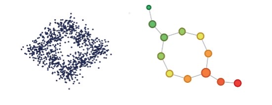
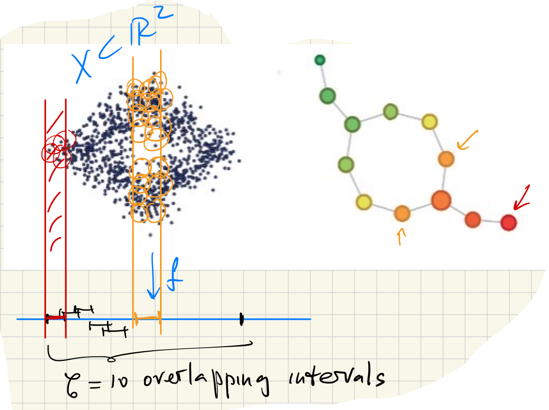
Consider data points sampled around the unit circle. Let $f:{ℝ}^2\to ℝ$ by $f(x,y)=x$. Suppose the image $f(X)$ is covered by small overlapping intervals of equal length. Mapper recovers the topology of the circle:

If we had used a simple cover (single interval), the Mapper graph would have no edges and thus would not express the circle’s topology.

(Rabadan-Blumberg 2020)

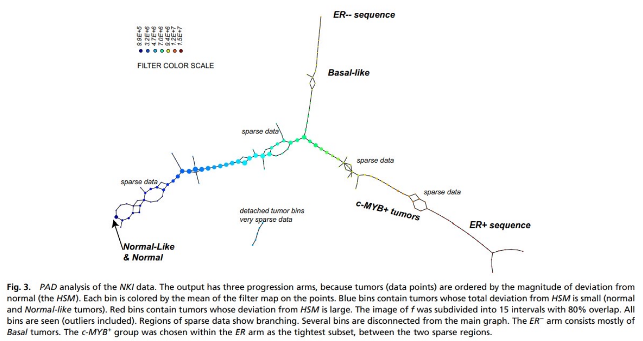
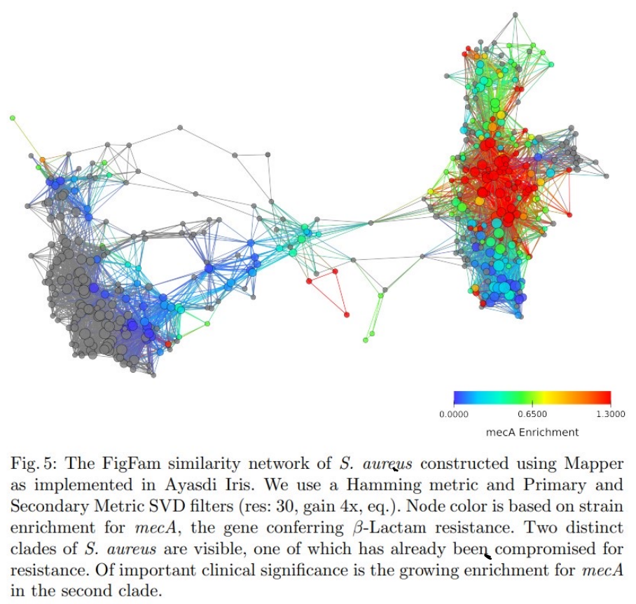
(Nikolau-Levine 2011)

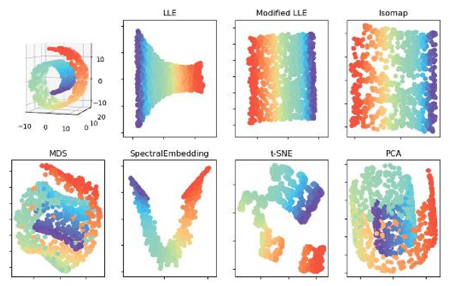
Dimensionality reduction and manifold learning

These techniques work well if the given data happens to lie near a lower-dimensional vector subspace or submanifold of the original space.

Foundational algorithms are

• PCA “principle component analysis” — vector subspaces
  • starts with $X\subset {ℝ}^n$ a finite metric space (point-cloud data)
• MDS “multidimensional sampling” — manifold subspaces
  • starts with arbitrary metric space $(X,d)$

Goal:

Given (small) $k\in {\mathbb{Z}}_{\ge 0}$, find an optimal map $\theta :X\to {ℝ}^k$ which in some sense represents the structure of the data by minimizing the error:

$$ℰ=\sum _{x_i,x_j\in X}(d_X(x_i,x_j)-d_{{ℝ}^k}(\theta (x_i),\theta (x_j)){)}^2$$

10 Theory - PCA

Let $M$ be an $n\times n$ matrix with eigenvalues ${\lambda }_i$ and eigenvectors ${𝐯}_i$, so $M{𝐯}_i={\lambda }_i{𝐯}_i$.

Recall that if $M$ is symmetric, we know that ${\lambda }_i\in ℝ$ and

$${\lambda }_i\ne {\lambda }_j⟹{𝐯}_i⟂{𝐯}_j$$

For PCA, we start with $X=\{{𝐱}_1,{𝐱}_2,\dots ,{𝐱}_3\}\subset {ℝ}^n$. Fix $k\in {\mathbb{Z}}_{\ge 0}$ small.

The goal is to find an “optimal” linear map $\theta :{ℝ}^n\to {ℝ}^k$ which distorts distances between data points as little as possible. (Minimal mean-square error.)

PCA Algorithm: (1) Normalization

Consider $\mu =\frac{1}{n}{\sum }_i{𝐱}_i$ and let ${\widetilde{𝐱}}_i={𝐱}_i-\mu$.

(2) Covariance matrix

Define the covariance matrix $C$:

$$C=\frac{1}{n}\sum _i{\widetilde{𝐱}}_i{\widetilde{𝐱}}_i^{𝖳}$$

Note that $C_{jk}={𝐱}_j\cdot {𝐱}_k$. Then, since each summand of $C$ is symmetric, $C$ must be symmetric.

(3) Eigenvalues

Compute the top (largest) $k$ eigenvalues of $C$.

If these are pairwise distinct, the corresponding eigenvectors are all linearly independent, so they span a $k$-dimensional linear subspace $V$.

Consider the orthogonal projection $\theta :{ℝ}^n\to V$.

(Note: one must somehow identify $V$ with ${ℝ}^k$ first.)

If some eigenvalue ${\lambda }_j$ has multiplicity, then consider the corresponding eigenspace $V_j$.

Theorem:

The outcome of this algorithm is an optimal $\theta$ which minimizes the error $ℰ$.

(In the context of PCA or MDS, in fact.)

Combining techniques

It is often reasonable to combine techniques discussed thus far.

For example, the outcome of PCA/MDS may be fed into Mapper; a coordinate project in the PCA output may be used as the filter function.

11 Theory - MDS

Multi-dimensional scaling starts with an arbitrary finite metric space $(X,d)$, and attempts to embed this in ${ℝ}^k$ in a way that is optimal in the sense of minimizing $ℰ$. This is done as follows:

(1) Metric matrix:

$$D_{ij}=d_X({𝐱}_i,{𝐱}_j)$$

(2) $H$ and $Z$

Let $H$ be the matrix $H=I-\frac{1}{n}\mathrm{𝟏}$ where $\mathrm{𝟏}$ is the matrix with all entries $1$.

Let $Z$ be the matrix $Z=-\frac{1}{2}HDH$.

(This step centers the result at the origin.)

(3) Define $\theta :X\to {ℝ}^k$:

Create a matrix $A$ with columns the eigenvectors ${𝐯}_j$, normalized so that $||{𝐯}_j|{|}^2={\lambda }_j$. Then:

$$\theta (x_i)=i^{\text{th}}\text{ row of }{A}^{𝖳}$$

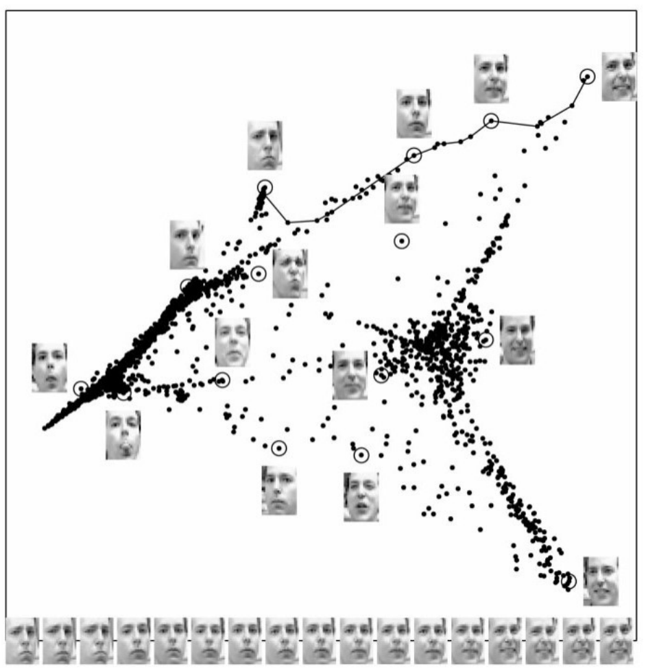
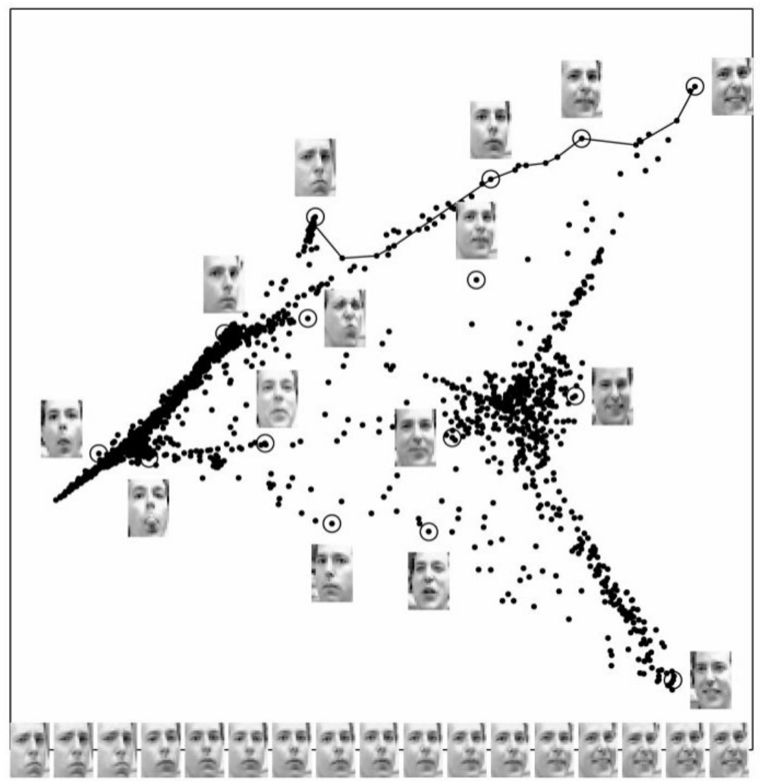
12 Theory - Isomap manifold learning

The given data is aligned along a non-linear subspace of ${ℝ}^n$.

This method is used in facial recognition, for example.

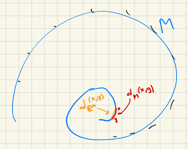
We are assuming that the data lies along (very near) a submanifold $M\subset {ℝ}^n$. This $M$ is assumed to have an “intrinsic” metric $d_M(x,y)$ for $x,y\in M$.

$$d_M(x,y)=\underset{\text{curves }\alpha }{\min }{\int }_0^1||\dot{\alpha }(t)||dt$$

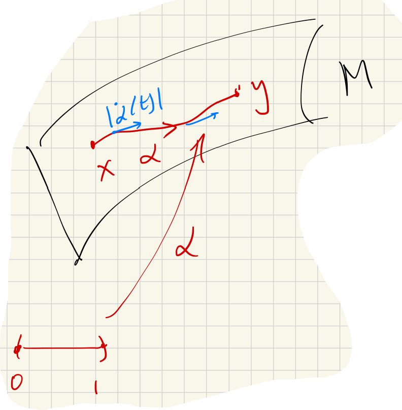
The idea of isomap is that, assuming $M\subset {ℝ}^n$ is smoothly embedded, there is a scale at which

$$d_M(x,y)\sim d_{{ℝ}^n}(x,y)$$

Isomap description in detail:

Let us be given $X=\{{𝐱}_1,\dots ,{𝐱}_m\}\subset {ℝ}^n$, as well as a scale $\epsilon >0$ and a target dimension $k$.

Isomap procedure

(1) Build weighted graph $G$:

• Vertices: the points ${𝐱}_1,\dots ,{𝐱}_m$
• Edges: join ${𝐱}_i$ to ${𝐱}_j$ when $d({𝐱}_i,{𝐱}_j)<\epsilon$
• Weights: the distances $w_{ij}=d({𝐱}_i,{𝐱}_j)$

(2) New metric space $(X^{\prime },d_{X^{\prime }})$:

Same points, new distances:

$$d_{X^{\prime }}({𝐱}_i,{𝐱}_j)=\underset{\begin{array}{c}\text{paths }{𝐱}_i\\ \text{ to }{𝐱}_j\text{ in }G\end{array}}{\min }\sum \text{path weight}$$

(Use Dijkstra’s Algorithm to compute the minimal path.)

(3) Apply PCA/MDS:

Find an optimal map $\theta :X^{\prime }\to {ℝ}^k$.

Isomap - single chart

Isomap is most effective when the manifold can be covered by a single chart and the algorithm effectively “flattens” and “unrolls” the space.

It is less effective for manifolds with topology. For example, when applied to ${𝕊}^2\subset {ℝ}^3$, the output of isomap is a flat disk.

(Rabadan-Blumberg 2020)

13 Theory - Local Linear Embedding (LLE)

LLE is a variation of isomap manifold learning that is “locally linear.” It does not attempt to preserve the metric globally. The algorithm is a little more efficient than isomap as well.

LLE Procedure

Suppose we are given the data set $\{{𝐱}_1,\dots ,{𝐱}_m\}\subset {ℝ}^n$, the target dimension $k\in \mathbb{N}$ and a “neighborhood size” $K$.

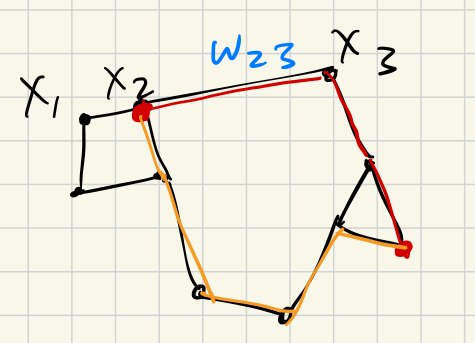
(1) Find minimizer weights:

For each ${𝐱}_i$, find weights $w_{ij}$ that minimize the error:

$$ℰ=\sum _i{({𝐱}_i-\sum _j{w}_{ij}{𝐱}_j)}^2$$

subject to the constraints:

$$\{\begin{array}{cc}{w}_{ij}& =0\text{ if }{𝐱}_i,{𝐱}_j\text{ are NOT }K\text{-neighbors}\\ & \\ \sum _j{w}_{ij}& =1\end{array}$$

The weights determine approximations of a point using the plane that best fits its neighbors. If the manifold is actually linear around a point, the error at that point will be zero.

(2) Use minimizer weights to recover points:

Find points $\{y_1,\dots ,y_m\}\subset {ℝ}^k$ that minimize the error:

$$ℰ=\sum _i{(y_i-\sum _j{w}_{ij}{y}_j)}^2$$

The new embedding is $\theta :x_i⟼y_i$.

Locality

The Isomap and LLE algorithms are local, meaning that the output $\theta (x)$ is determined by the data around $x$. Data points far from $x$ have no effect on $\theta (x)$.