TDA Notes - Unit 05

Laplacian eigenmaps

The Laplace operator on smooth functions on may be written in a variety of ways:

We would like to extend the concept of to

1. smooth manifolds (coordinate independent version)
2. graphs (combinatorial version)

01 Theory - Laplace-Beltrami operator

The extension of the concept of to smooth manifolds is called the Laplace-Beltrami operator. It is still defined as the divergence of the gradient, but these too must be upgraded to the context of manifolds.

Write for the space of smooth functions . Write for the space of differential -forms on . The exterior derivative is a map:

and the co-differential is a map:

(It is defined using the Hodge star operator.) Then .

The spectrum of is the set of eigenfunctions , meaning functions satisfying:

for some .

If you know the complete spectrum of , then you know a lot about the shape of (although you may not be able to recover completely).

02 Theory - Laplacian for graphs

In spectral graph theory one studies the spectrum of a combinatorial extension of the Laplacian concept to a graph.

We start with a weighted graph:

• Vertices
• Edges with weights

The adjacency matrix is the matrix for off-diagonal elements, and zeros on the diagonal. (No self-loops.)

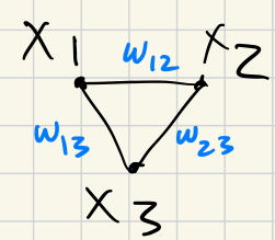
The graph Laplacian is the matrix with off-diagonal, and the diagonal entries given as follows:

Then:

Explanation:

For a graph , let

• be the vector space with edges of as basis
• be the vector space with vertices of as basis

Then define

by .

There is an adjoint (transpose) map .

Laplacian eigenmaps process

Let us be given a scale and a target dimension .

Form a weighted graph:

• Vertices
• Edge weights: as follows:

Let and by . The graph Laplacian is .

Consider the matrix with columns given by eigenvectors corresponding to the -largest eigenvalues of . The rows of this matrix define points . Define by assigning

This definition of minimizes the error:

Given the definition of , this error penalizes most strongly nearby points that are sent to distant points .

The Laplacian eigenmaps process does not work well for spheres and other noncontractible spaces that are not covered by a single coordinate chart.

UMAP

Uniform Manifold Approximation and Prediction

The goal of UMAP is to rebuild the data in a high space as:

• Low-dimensional manifold
  • The data is first cast as a weighted graph (1-dimensional)
• Uniform sampling assumption
  • Dense clusters are spread apart and sparse areas contracted

03 Theory - UMAP process

We are given a data cloud , and a neighbor-count .

(1) Create weighted partial graphs local to each data point:

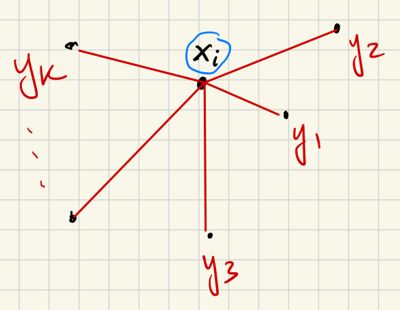
For each point , define weights as follows:

• Set .
• All are infinitely far from each other: for .
• For :
  • Require that is proportional to ,
  • Require that .

That is, the nearest neighbor is placed at distance from , and the other neighbors are made closer to by the distance removed. For each fixed , the collection encodes metric structure of the original data near but with the closest point substituted for .

The weight is supposed to be interpreted as the probability that the point will lie in the same cluster as the point .

From these requirements it is possible to deduce a formula for , as follows:

Set . (Distance to the closest neighbor.) For each , solve for such that:

The idea is that for the closest neighbor , the weight should be the highest; the weight should decrease for neighbors that are farther away.

---

(2) Glue partial metrics into a single weighted graph:

Now we define a single weighted graph with vertices the points and weights coming from the set of partial graphs defined in Step (1).

Observe that a given pair of vertices could appear with finite distance in at most two partial graphs. The relation of being “nearest neighbor” is not in general symmetric:

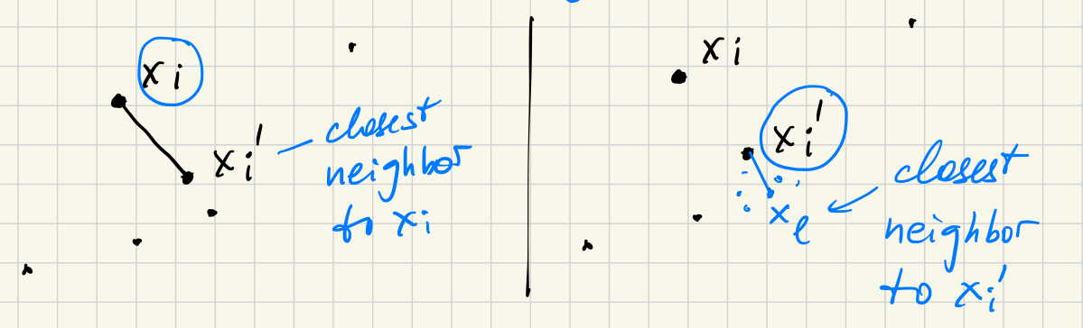
Now, let us be given a pair of vertices .

If this pair appears (with finite weight) in only one partial graph, give the pair a weighted edge in the total graph with the same weight it had in that partial graph.

If this pair appears in two partial graphs, then is the center point in one of them and is the center in the other.

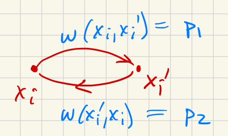
We combine the weights as follows:

• Let
• Let

Then the weight on the pair shall be defined as:

Now we have defined a total weighted graph that combines the information from all the weighted partial (local) graphs.

---

(3) Embed the total weighted graph in a lower-dimensional space as a weighted graph .

This can be done with standard techniques that we don’t cover here. Briefly:

Start with the spectral graph embedding. Edge weights for edge are in and in . Cross-entropy formula:

Use this cross-entropy as a cost function and perform stochastic gradient descent to minimize the cost.

04 Theory - Gradient descent

Suppose we are given a cost function .

Given any , the gradient of , written , is the direction of the largest rate of change of .

Smallest rate of change is .

05 Illustration

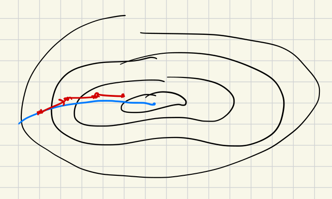
UMAP is based on an assumption that the data samples uniformly from a manifold.

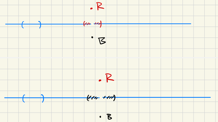
Hausdorff manifolds?

Consider with the standard non-Hausdorff metric:

So the points and cannot be separated by a disjoint neighborhood.

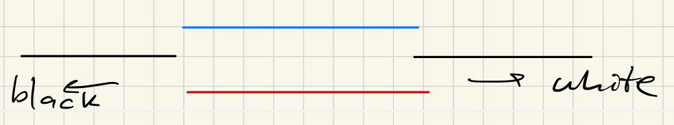
But this can actually happen with data! Suppose flowers come in two colors, red and blue, but the value (lightness) ranges from very dark (black) to very light (white):

06 Illustration

(Böhm et al. 2022)