Vector Calculus - Packet 05

Parametric space curves: differentiation

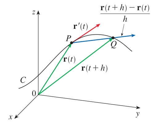
A vector-valued parametric curve in may be given in terms of component functions by . When the component functions are differentiable, then is also said to be differentiable, and the derivative function is . Applying the same logic repeatedly, one obtains higher derivatives .

Example

Derivative of vector function, constant basis

Consider . Find and .

Solution: Differentiation is given componentwise, so we can treat the basis vectors as constants and differentiate their coefficients: and .

Derivative rules for parametric space curves

Given vector functions, and a scalar, and a scalar function (all differentiable), then the standard derivative rules for algebraic compositions of functions determine rules applying to vector operations: e

• Sums:
• Constants:
• Scalar products:
• Chain rule:

Moreover, by considering the component formulas for vector products, one finds derivative rules for vector products analogous to the rule for a scalar product:

• Dot product rule:
• Cross product rule:

Exercise 05A-01

Parametric curve: derivative rules for vector products

Use the algebraic properties of dot and cross product to prove the derivative product rules without using the component descriptions of those products. (Imitate the proof of the standard product rule.)

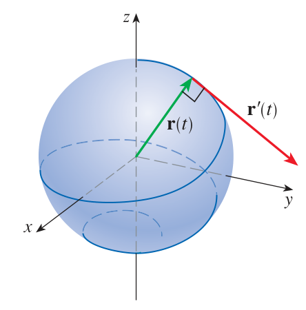
Constant norm vector functions When a vector-valued parametric function has constant norm , the vector is necessarily perpendicular to its own derivative:

This fact is often applied to the case of a unit vector. Intuitively, a unit vector gives a direction as a point on the unit sphere. An infinitesimal change of this direction will lie in the tangent plane to the sphere, which is perpendicular to the sphere, and thus perpendicular to the original vector.

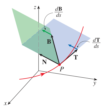
Tangent and normal vectors

The tangent vector of a parametric curve is just the derivative of as a vector-valued parametric function. It is tangent to the curve:

When the curve is non-stationary, i.e. , then its tangent vector determines a unit tangent vector which is typically written . This vector represents the direction of travel of a particle traversing the curve.

When the component functions are twice differentiable, the unit tangent has a derivative . Where the curve is non-straight, i.e. , then determines a unit normal vector , also called the principal normal vector.

and are perpendicular Since has a constant norm of one, we know that at all times.

Exercise 05A-02

and for a circle

Compute and for the circle in the -plane given parametrically by .

Distance traveled, speed

To improve the expression of various formulas, we use the notation:

The distance traveled function is given for a parametric curve in by:

It follows from the Fundamental Theorem of Calculus that:

This quantity is called the speed of travel at time .

Exercise 05A-03

Derivative of reparametrized curve

Suppose is a parametric curve, and is a function of another parameter . Under what condition on does the composite curve have unit speed everywhere?

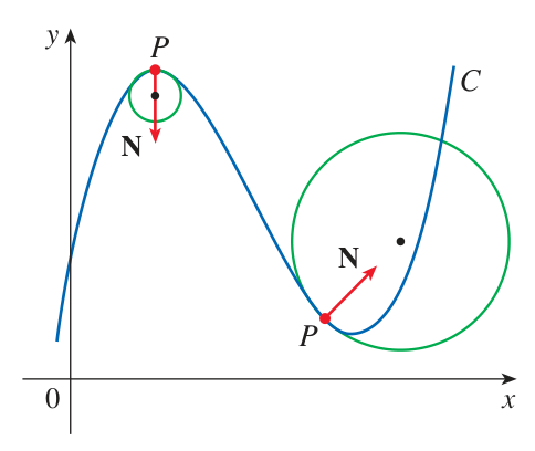
Curvature

The curvature of a space curve is defined as the rate of change of the unit tangent vector with respect to distance traveled.

For curves in the plane, a single quantity, the angle of inclination , is sufficient to characterize the heading direction, and the curvature is given by . For curves in space, the unit vector plays the role of , giving the heading direction. (In spherical coordinates, a point on the unit sphere is determined by two angle quantities , .) The rate of change of heading is best described as a vector quantity whose norm gives the curvature:

The curvature quantifies a geometrical property of the curve image, and it does not depend on the parametrization. This follows because and are both functions of the curve image. (Plus a chosen direction of travel along the curve that determines signs, but the sign of cancels the sign of ). A point on the curve may be specified by the parameter or by the arc length , so may be considered a function of or of .

Using the fact that , we find that the rate of change of the unit tangent with respect to the parameter can be expressed in terms of speed, curvature, and the unit normal:

Exercise 05A-04

Curvature of a line

Use for a vector-valued parametric line. Compute the curvature of this line using the definition of curvature.

Exercise 05A-05

Curvature of a circle

Write component formulas for a vector-valued parametric circle of radius in . Compute the curvature of this circle using the definition of curvature.

Acceleration decomposition

The acceleration vector of is defined as its second derivative with respect to time: .

Since is defined using , and is defined using , we expect a relation between and . Indeed we have:

This follows because , so the product rule gives:

Efficient curvature formula The quantity in the denominator of often makes the derivative annoying to compute. It is possible to avoid this derivative by using further reasoning to develop an alternate formula for . First, observe that:

Since is a unit vector, it follows by taking norms that:

Efficient formula for The decomposition of can also be used to give an efficient formula for :

We can see this by multiplying the decomposition by :

Dividing both sides by the norm gives the desired formula.

Exercise 05B-01

Curvature of a helix

Compute the curvature of the helix given parametrically by using the efficient formula. Also compute the unit tangent and principal normal vectors, and . Compute once using the definition, and again using the efficient formula.

Exercise 05B-02

Curvature of a graph

Use the efficient formula for curvature to derive a formula for the curvature of the graph of a function , namely the points satisfying . Start by finding a parametric curve whose image is this graph.

Exercise 05B-03

Normal vector to at

Compute the principal normal using the efficient formula for the parametric curve given by at the point .

Acceleration decomposition Given that and are orthogonal unit vectors and is a linear combination of them, it is appropriate to name the components of according to the decomposition:

with and . So is the component of acceleration in the direction of travel, which by the definition is also just the rate of change of the scalar speed with respect to time; and is the component of acceleration in the normal direction, perpendicular to the direction of travel.

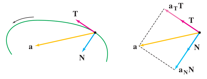
Acceleration lies in span of and

The fact that can be written as a linear combination of and says something about . In fact it gives a way to characterize : it is the unique direction perpendicular to that is determined by the part of perpendicular to .

Exercise 05B-04

Acceleration on a circle

Write a parametric curve traversing a circle of radius in at constant speed. Compute the decomposition of acceleration into components: .

Going deeper

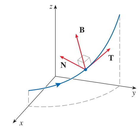
The space of vectors perpendicular to is a plane, so is not unique with the property that . It is unique in containing the new direction of . The plane given by all linear combinations of and is called the osculating plane.

Another unit vector may be defined by , and we also have . It is called the ‘binormal’ vector. The collection of pairwise orthogonal unit vectors forms a special basis naturally arising from the parametric curve which is called the ‘Frenet-Serret frame’, or sometimes the ‘ frame’.

Frenet-Serret graphics on Wikipedia

Parametric space curves: integration

Arc length parametrization

A parametric curve is said to have unit speed when .

Another description with the same meaning is to say that has an arc length parametrization. This terminology is used because the distance-traveled function is when .

Typically a parametric curve with arc length parametrization is written using the letter ‘’ for the parameter, as in , to emphasize the fact that the parameter also measures the distance traveled along the curve.

The distance traveled is also the only natural parameter, in that it is determined by the image curve in , whereas any other parameter , for , suffers from an undesirable arbitrariness. (For example, what geometric reason could be given to choose instead of ?)

A consequence of the fact that is geometrically natural is that arc length parametrizations are very useful in abstract mathematics, where arguments about geometrical structure are sought. Unfortunately it is often impracticable to create arc length parametrizations with explicit formulas, so they are less useful in practical applications. There are some exceptions.

Example

Arc length parametrization of a line.

Calculate an arc length parametrization of the line in the plane given by .

Solution: We create a natural parametrization of the line using . Observe that and . Using the definition of , we then find:

Solving for , we find . Plugging this into the original parametrization, obtain:

Exercise 05B-05

Compute arc length parametrization of a helix

Calculate an arc length parametrization of the helix given parametrically by . Start by computing the distance-traveled function , and then find its inverse function , and plug this into the original parametrization.

Problems due 23 Sep 2023, 8:00pm

Problem 05-01

Tangent lines to parametric curves

For the following parametric curves, find a parametrization of the tangent line to the curve at the given time:

• (a) at
• (b) at
• (c) at

Problem 05-02

Natural vectors and curvature

For the following parametric space curves, compute , , , and . Decompose in terms of and .

• (a)
• (b)

Problem 05-03

Arc length parametrization of

Calculate an arc length parametrization of the plane curve parametrized by .

Problem 05-04

Quadratic curve is planar

The component functions for a parametric space curve are quadratic polynomials in the parameter . Show that this space curve lies in a plane.