Vector Calculus - Packet 06

Parametric space curves: vector integration

Vector integrals

A parametric space curve $𝐫(t)=(x(t),y(t),z(t))$ has a definite vector integral that is defined componentwise:

$${\int }_a^b𝐫(t)dt=({\int }_a^{b}x(t)dt,{\int }_a^{b}y(t)dt,{\int }_a^{b}z(t)dt).$$

The vector integral relates directly to the componentwise derivative ${𝐫}^{\prime }(t)$ by a vector form of the Fundamental Theorem of Calculus:

$${\int }_a^b𝐫(t)dt=𝐑(b)-𝐑(a)$$

where $𝐑(t)$ is a vector antiderivative of $𝐫(t)$, meaning that ${𝐑}^{\prime }(t)=𝐫(t)$.

Using the standard calculus argument applied to each component separately, one has the fact that:

$${𝐑}_1^{\prime }(t)={𝐑}_1^{\prime }(t)⟹{𝐑}_1(t)={𝐑}_1(t)+𝐜,$$

where $𝐜=(c_1,c_2,c_3)$ is some constant vector. This means that if ${𝐑}^{\prime }(t)=𝐫(t)$, so $𝐑(t)$ is a particular antiderivative of $𝐫(t)$, then the general antiderivative is given by $𝐑(t)+𝐜$ for a constant vector $𝐜$. So we can write the indefinite vector integral:

$$\int 𝐫(t)dt=𝐑(t)+𝐜.$$

The vector integral ${\int }_a^{b}v(t)dt$ may be interpreted as the total motion of a particle whose velocity is given by $v(t)$.

Integration for components, not coordinates

If a parametric curve is given using spherical coordinate functions, for example $(r(t),\theta (t),\phi (t))$, then the componentwise derivatives and integrals do not have vector interpretations as tangent vector and total motion vector. The meaning of vector derivative and integral depends on the componentwise addition and scaling operations applicable to vectors.

Example

Indefinite vector integral calculation

Problem: Compute the indefinite vector integral: $\int (e^t,t^{\frac{1}{2}},\cos (t))dt$.

Solution: The vector integral is given by computing ordinary integrals in each component. We have:

$$\begin{array}{cc}\int (e^t,t^{\frac{1}{2}},\cos (t))dt& =(\int e^{t}dt,\int t^{\frac{1}{2}}dt,\int \cos (t)dt)\\ & =(e^t+c_1,\frac{2}{3}{t}^{\frac{3}{2}}+c_2,\sin (t)+c_3)\\ & =(e^t,\frac{2}{3}{t}^{\frac{3}{2}},\sin (t))+𝐜.\end{array}$$

Exercise 06A-01

Indefinite vector integrals

Compute the indefinite vector integrals:

• (a) $\int \frac{1}{1+t^2}{𝐞}_{𝐢}+t{e}^{t^2}{𝐞}_{𝐣}+\sqrt{t}{𝐞}_{𝐤}dt$
• (b) $\int (t\cos (t^2),t^{-1},{\sec }^2(t))dt$

Exercise 06A-02

Definite vector integrals

Compute the definite vector integrals:

• (a) ${\int }_a^b(1,t^2,\sin (t))dt$
• (b) ${\int }_0^1(\frac{1}{1+s^2},\frac{s}{1+s^2})ds$
• (c) ${\int }_0^{1}t{e}^{-t^2}{𝐞}_{𝐢}+t\ln (t^2+1){𝐞}_{𝐣}dt$
• (d) ${\int }_0^t(3s,6s^2,9)ds$

Position, velocity, acceleration

If the position of a moving particle is identified using the vector-valued parametric function $𝐫(t)$, then its velocity is given by ${𝐫}^{\prime }(t)$ and its vector acceleration is ${𝐫}^{\prime \prime }(t)$.

The definite vector integral reverses this progression. We have ${\int }_a^b{𝐫}^{\prime \prime }(t)dt={𝐫}^{\prime }(b)-{𝐫}^{\prime }(a)$, the total change in velocity over the time interval $a\le t\le b$. Similarly ${\int }_a^b{𝐫}^{\prime }(t)dt=𝐫(b)-𝐫(a)$, the total change in position over the same interval.

Particle position from velocity: differential equation

Problem: Suppose that the path of a particle is given by $𝐫(t)$ and that its velocity satisfies ${𝐫}^{\prime }(t)=(1-6\sin (3t),4t,e^t)$, and suppose the particle passes through the point $(\mathrm{4,1,2})$ at $t=0$. Find $𝐫(t)$ and use your formula to find the position of the particle at $t=2$.

Solution: By taking the indefinite vector integral of both sides of ${𝐫}^{\prime }(t)=(1-6\sin (3t),4t,e^t)$, we obtain the general solution:

$$𝐫(t)=(t+2\cos (3t),2t^2,e^t)+𝐜.$$

We can solve for $𝐜$ by setting $𝐫(0)=(\mathrm{4,1,2})$:

$$(\mathrm{4,1,2})=(\mathrm{2,0,1})+𝐜$$

so $𝐜=(\mathrm{2,1,1})$ gives the particular solution satisfying the initial condition $𝐫(0)=(\mathrm{4,1,2})$.

Exercise 06A-03

Differential equations

For the differential equations below, find the general solution, and find the particular solution that satisfies the given initial condition:

• (a) $\frac{d𝐫}{dt}=(1-3t,4t),𝐫(0)=(\mathrm{3,1})$
• (b) ${𝐫}^{\prime }=t^2{𝐞}_{𝐢}+5t{𝐞}_{𝐣}+{𝐞}_{𝐤},𝐫(1)={𝐞}_{𝐣}+2{𝐞}_{𝐤}$
• (c) ${𝐫}^{\prime \prime }(t)=(e^{2t-2},t^2-\mathrm{1,2}),𝐫(0)=(\mathrm{1,0,0}),{𝐫}^{\prime }(0)=(\mathrm{0,1,0})$

Kepler’s Law of Ellipses

Isaac Newton’s laws of motion were used to derive and explain Johannes Kepler’s observed law that planets orbit the sun with elliptical orbits. We can use vector integration to solve a differential equation coming from Newton’s laws to give a modern derivation of this law of elliptical orbits.

Set the sun at the origin $(\mathrm{0,0,0})$, and let $𝐫(t)$ describe the orbit of some planet. Let $G$ be the gravitational constant, $M$ the mass of the sun, and $m$ the mass of the planet. Let $𝐅(t)$ be the total force vector on the planet. By Newton’s law of gravitation:

$$𝐅=-\frac{GMm}{|𝐫{|}^2}{𝐞}_{𝐫}.$$

By Newton’s law of motion, $𝐅=m𝐚$ where the acceleration is $𝐚(t)={𝐫}^{\prime \prime }(t)$. By identifying the force in each equation, we obtain the vector differential equation:

$${𝐫}^{\prime \prime }(t)=-\frac{GM}{|𝐫(t){|}^2}{𝐞}_{𝐫}(t)=-\frac{GM}{|𝐫(t){|}^3}𝐫(t).$$

Exercise 06A-04

Prepare to explain the following reasoning in class:

Planet motion stays in some plane: $𝐫\times {𝐫}^{\prime }=𝐧$

Consider the following calculation:

$$\begin{array}{cc}\frac{d}{dt}(𝐫\times {𝐫}^{\prime })& ={𝐫}^{\prime }\times {𝐫}^{\prime }+𝐫\times {𝐫}^{\prime \prime }\\ & =0+𝐫\times (-\frac{GM}{|𝐫{|}^3}𝐫)=0.\end{array}$$

By integrating both sides of this vector equation, we find $𝐫\times {𝐫}^{\prime }=𝐧$ for some constant vector $𝐧$. So $𝐧$ is perpendicular to $𝐫(t)$ for all $t$, which means $𝐫(t)$ lies in the plane through the origin with normal vector $𝐧$.

Exercise 06A-05

Prepare to explain the following reasoning in class:

Equation to integrate: ${({𝐫}^{\prime }\times 𝐧)}^{\prime }=GM{𝐞}_{𝐫}^{\prime }$

Next we verify this equation. The product rule gives ${({𝐫}^{\prime }\times 𝐧)}^{\prime }={𝐫}^{\prime \prime }\times 𝐧$. Now compute this using the vector differential equation and the definition of $𝐧$:

$${𝐫}^{\prime \prime }\times 𝐧=-\frac{GM}{|𝐫{|}^3}𝐫\times (𝐫\times {𝐫}^{\prime }).$$

Expand the triple product with the Lagrange triple product identity $𝐚\times (𝐛\times 𝐜)=𝐛(𝐚\cdot 𝐜)-𝐜(𝐚\cdot 𝐛)$, and let $r=|𝐫|$, so $𝐫=r{𝐞}_{𝐫}$, and calculate:

$$\begin{array}{cc}-\frac{GM}{|𝐫{|}^3}𝐫\times (𝐫\times {𝐫}^{\prime })& =-\frac{GM}{r^3}(𝐫(𝐫\cdot {𝐫}^{\prime })-{𝐫}^{\prime }(𝐫\cdot 𝐫))\\ & =-\frac{GM}{r^3}(r{𝐞}_{𝐫}(r{𝐞}_{𝐫}\cdot (r^{\prime }(t){𝐞}_{𝐫}+r{𝐞}_{𝐫}^{\prime }))-(r^{\prime }(t){𝐞}_{𝐫}+r{𝐞}_{𝐫}^{\prime })r^2)\\ & =-\frac{GM}{r}({𝐞}_{𝐫}(r^{\prime }(t)+0)-r^{\prime }(t){𝐞}_{𝐫}-r{𝐞}_{𝐫}^{\prime })\\ & =GM{𝐞}_{𝐫}^{\prime }.\end{array}$$

Exercise 06A-06

Prepare to explain the following reasoning in class:

Result of integration: ${𝐫}^{\prime }\times 𝐧=GM{𝐞}_{𝐫}+𝐜$

Take the indefinite vector integral on both sides of ${({𝐫}^{\prime }\times 𝐧)}^{\prime }=GM{𝐞}_{𝐫}^{\prime }$ and obtain ${𝐫}^{\prime }\times 𝐧=GM{𝐞}_{𝐫}+𝐜$ where $𝐜$ is some constant vector.

Notice that $𝐜⟂𝐧$ by taking $-\cdot 𝐧$ on both sides of the stated equation, using that ${𝐞}_{𝐫}⟂𝐧$. This means $𝐜$ lies in the same plane of the orbit that $𝐫(t)$ lies in.

Let $c:=|𝐜|$ and let $\theta (t)$ be the angle between $𝐫(t)$ and $𝐜$ in the plane perpendicular to $𝐧$. Also let $n:=|𝐧|$.

Exercise 06A-07

Prepare to explain the following reasoning in class:

Triple product for scalar equation

We take the dot product $𝐫\cdot -$ on both sides of the previous stated equation, and rearrange the triple product, in order to find a scalar equation:

$$\begin{array}{cc}𝐫\cdot ({𝐫}^{\prime }\times 𝐧)& =GM𝐫\cdot {𝐞}_{𝐫}+𝐫\cdot 𝐜\\ 𝐧\cdot (𝐫\times {𝐫}^{\prime })& =GMr+rc\cos (\theta ).\end{array}$$

Since $𝐫\times {𝐫}^{\prime }=𝐧$ and $𝐧\cdot 𝐧=n^2$, we have:

$$n^2=r(GM+c\cos (\theta )),$$

so:

$$r=\frac{n^2}{GM}\left(\frac{1}{1+e\cos (\theta )}\right),$$

where $e:=\frac{c}{GM}$ is defined to simplify the expression. This, now, is the polar equation of an ellipse with eccentricity $e$.

Line integrals I: scalar fields

A scalar line integral is the integral of a function over the length of a curve.

A line integral sums the values of a scalar function on space multiplied over the length of some curve in space. This would be an ordinary integral if the curve were stretched out onto an $x$-axis and the function values plotted on the $y$-axis.

Line integral with parametrization $𝐫(t)$ Suppose $f:{ℝ}^3\to ℝ$ is a function on space with values given by $f(x,y,z)$, where $(x,y,z)$ are the coordinates of the input point in space. Suppose a curve $C$ is the image of a parametric curve given with component functions by $𝐫(t)=(x(t),y(t),z(t))$, and assume $C$ is traversed exactly once by $𝐫(t)$. Then we compute the line integral of $f$ over $C$ using the formula:

$${\int }_{C}f(x,y,z)ds={\int }_a^{b}f(𝐫(t))\cdot |{𝐫}^{\prime }(t)|dt.$$

This formula uses our expression for infinitesimal distance traveled:

$$ds=|{𝐫}^{\prime }(t)|dt=\sqrt{x^{\prime }{(t)}^2+y^{\prime }{(t)}^2+z^{\prime }{(t)}^2}dt.$$

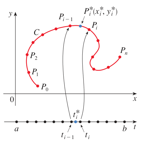
Rigorous definition idea A rigorous definition of the line integral ${\int }_{C}fds$ would divide the curve $C$ into $n$ segments joined at the points $(x_i,y_i,z_i)$, with segment length $\mathrm{\Delta }{s}_i$, then take the Riemann sum:

$$\sum _{i=1}^{n}f(x_i,y_i,z_i)\mathrm{\Delta }{s}_i,$$

and finally take the limit as the number of segments goes to infinity.

Line integral with arc length parametrization If we start with a curve $𝐫(s)$ parametrized by arc length, the line integral is very simply given by:

$${\int }_{C}fds={\int }_a^{b}f(𝐫(s))ds,$$

where $f$ is a scalar function of points in ${ℝ}^3$.

In fact, the line integral ${\int }_{C}fds$ is sometimes called the line integral with respect to arc length.

Line integral with respect to $x$, $y$, or $z$ A related construction is the line integral with respect to some coordinate. For example, the line integral of $f$ over a curve $C$ with respect to $x$ is given by the formula:

$${\int }_{C}fdx={\int }_a^{b}f(𝐫(t))\cdot x^{\prime }(t)dt.$$

Sometimes a sum of such integrals is written with shorthand notation as a single integral:

$${\int }_{C}fdx+gdy={\int }_a^{b}f(𝐫(t))\cdot x^{\prime }(t)+g(𝐫(t))\cdot y^{\prime }(t)dt.$$

When $C$ is traversed by $𝐫(t)$, this shorthand can be remembered with formulas using Leibniz notation:

$$dx=x^{\prime }(t)dt,dy=y^{\prime }(t)dt,dz=z^{\prime }(t)dt.$$

Example

Line integral in the plane

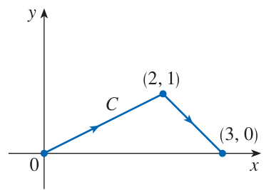
Problem: Compute the line integral:

$${\int }_{C}ydx+zdy+xdz$$

where $C$ is the line segment with endpoints $(\mathrm{2,0,0})$ and $(\mathrm{3,4,5})$. Solution: We use the formula $𝐫(t)=(1-t){𝐫}_0+t{𝐫}_1$ for a line passing through ${𝐫}_0$ and ${𝐫}_1$. This gives $𝐫(t)=(2+t,4t,5t)$. We also have $dx=dt$, $dy=4dt$, $dz=5dt$. Plugging everything in:

$${\int }_{C}ydx+zdy+xdz={\int }_0^{1}4t+5t\cdot 4+(2+t)\cdot 5dt={\int }_0^{1}10+29tdt=\mathrm{24.5.}$$

Example

Total mass of parabolic cable

Problem: A cable lies in ${ℝ}^2$ in the shape of a parabola satisfying $y=x^2$. The density of the cable is given by $\rho (x,y)=y/x$. Compute the total mass of the cable between $x=0$ and $x=4$. Solution: We use the parametrization of the parabola $P$ given by $𝐫(t)=(t,t^2)$ with $0\le t\le 4$. The total mass $M$ is given by the integral of density over the arc length of the curve:

$$M={\int }_P\rho (x,y)ds={\int }_0^4\rho (t,t^2)\cdot |(\mathrm{1,2}t)|dt={\int }_0^{4}t\sqrt{1+4t^2}dt\approx \mathrm{43.6.}$$

Exercise 06B-01

Line integrals with respect to arc length

Compute the line integrals of the given function over the specified curve:

• (a) $f(x,y,z)=x^2+y^2+z^2$ over the image of $𝐫(t)=(\cos (t),\sin (t),t)$ for $0\le t\le \pi$
• (b) $f(x,y)=\sqrt{1+9xy}$ over $y=x^3$ for $0\le x\le 1$
• (c) $f(x,y,z)=2x^2+8z$ over $𝐫(t)=(e^t,t^2,t)$ for $0\le t\le 1$

Exercise 06B-02

Electric potential from charged cable

The electric potential $V_p$ at a point $p=(a,b,c)$ in space is sourced by a charged circular wire with charge density $\rho (x,y,z)=(2-\frac{x}{R})$. The wire $C$ is located at $(R\cos (t),R\sin (t),0)$. The potential is given by the line integral:

$$V_p=k{\int }_C\frac{\rho (x,y,z)}{d_p}ds$$

where $k$ is a constant, $d_p$ is the distance from $p$ to $(x,y,z)$, and $C$ is a circle parametrized by $(R\cos (t),R\sin (t),0)$. Find the electric potential at the point $p=(\mathrm{0,0},c)$.

Exercise 06B-03

Line integrals compressed notation

Compute the following line integrals in the plane:

• (a) ${\int }_{C}ydx+zdy+xdz$ for $𝐜(t)=(2+t^{-1},t^3,t^2)$, $0\le t\le 1$
• (b) ${\int }_C\frac{-ydx+xdy}{x^2+y^2}$ for the line segment with endpoints $(\mathrm{1,0})$ and $(\mathrm{0,1})$

Exercise 06B-04

Line integrals in the plane

Compute the following line integral in the plane:

$${\int }_C(x+2y)dx+x^{2}dy$$

where $C$ is the following curve:

Problems due 30 Sep 2023, 8:00pm

By Kepler’s First Law, a planetary orbit is an ellipse, which lies in a plane. Assume this plane is the $xy$-plane, so $𝐫(t)=(x(t),y(t),0)$. Therefore $𝐧=𝐫\times {𝐫}^{\prime }$ may be written $𝐧=(\mathrm{0,0},n)$. Now rotate the $xy$-coordinates so that $𝐜=(c,\mathrm{0,0})$ and therefore the angle $\theta$ between $𝐫$ and $𝐜$ is also the polar angle of $𝐫$, so $𝐫(t)=(r(t)\cos (\theta (t)),r(t)\sin (\theta (t)),0)$ where $(r(t),\theta (t))$ describes the trajectory in polar coordinates in the $xy$-plane.

Problem 06-01

Kepler’s Second Law

This law states that the area swept out by a planet (in sectors drawn from the sun) is proportional to the time of travel (equal time, equal area), regardless of the point in the orbit. Verify this law in two steps:

• (a) Show that $𝐧=r^2{\theta }^{\prime }(t){𝐞}_{𝐤}$ and thus $n=r^2{\theta }^{\prime }(t)$.
• (b) Let $A(t)$ be the area swept out in the time interval $[t_0,t]$ for a fixed $t_0$. By calculating this area in polar coordinates, show that $A^{\prime }(t)=\frac{1}{2}{r}^2{\theta }^{\prime }(t)$, and thus $A^{\prime }(t)=\frac{1}{2}n$, a constant.

Problem 06-02

Kepler’s Third Law

This law states that the total orbit time squared is proportional to the major axis cubed. Verify this law in three steps:

Let $T$ be the total orbit time, and $2a$ the major axis, and $2b$ the minor axis.

• (a) Use the fact that $A^{\prime }(t)=\frac{1}{2}n$ to show $T=\frac{1}{n}2\pi ab$.
• (b) Show that $\frac{n^2}{GM}=\frac{b^2}{a}$ by converting the polar form of an ellipse to the rectangular form.
• (c) Show that $T^2=\left(\frac{4{\pi }^2}{GM}\right)a^3$, and note that $\left(\frac{4{\pi }^2}{GM}\right)$ does not depend on the planet.

$★$ Problem 06-03

Write and submit solutions to Exercises 06A-02, -03 and 06B-02, -04.