Vector Calculus - Packet 09

Partial Derivatives

Suppose we are given a function , written in terms of components by for each . Now let the second coordinate remain some arbitrary fixed value . This determines a function of one variable, , for each possible chosen .

We can take the derivative of in just as any other function of :

The resulting function of may be considered for various possible values of , i.e. the variation may be restored. This function of both and is called the partial derivative of with respect to . As with ordinary derivatives, a variety of notations is used:

The new symbol ‘ ’ is called “partial” and should be written differently from ‘ ’. This symbol indicates the function’s dependence on additional variables.

Functions of several variables may have partial derivatives in each of their variables. Thus, for above we also have or .

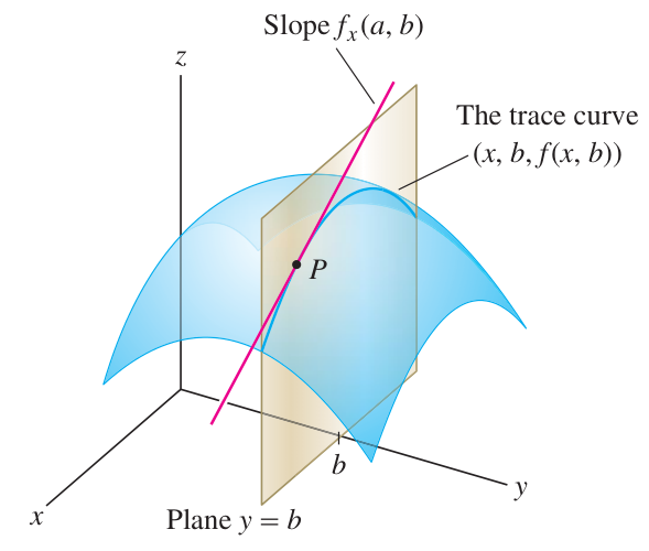
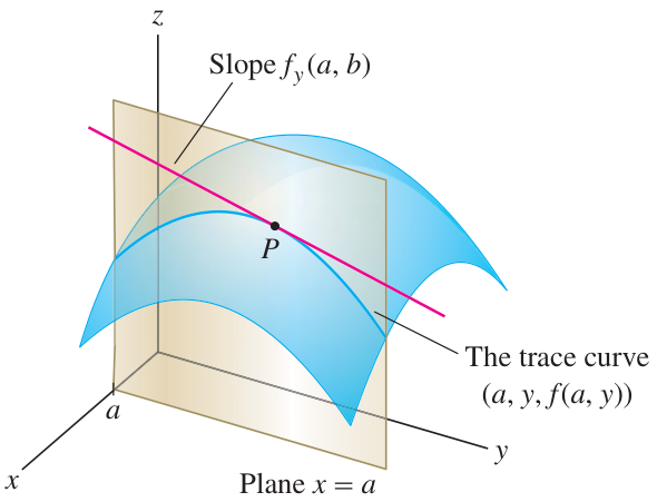
By interpreting the function as the “trace” of the function at a fixed value , one sees that the partial derivative gives the slope of the curve formed as the cross-section of the plane with the graph of , namely the surface : Similarly for the partial and the trace :

One can iterate partial derivatives and consider higher partials in the obvious manner. The notation indicates the “mixed partial” taken in first:

In principle, the double partials and could be different, but for nice functions they do agree by Clairaut’s Theorem:

Clairaut’s Theorem

Provided and exist and are continuous on a region , then on that region.

(Caveat: in the theorem, should be ‘open’ topologically: it should have the same dimension as the background and not include its boundary.)

Example

Partial derivatives of a monomial

Problem: Compute the partial derivatives of first and second order of the function . Solution: We have , , , , .

Exercise 09A-01

Partial derivatives of a composite

Let . Compute and .

Exercise 09A-02

Evaluate partial with four variables

Let

Calculate .

Exercise 09A-03

Higher order partials

Let .

• (a) Calculate the second-order partial derivatives of .
• (b) Calculate .

Exercise 09A-04

Clairaut: choose the order wisely!

Let . Compute in your head. (Explain it on paper!)

Continuity and differentiability: more complex in 3d!

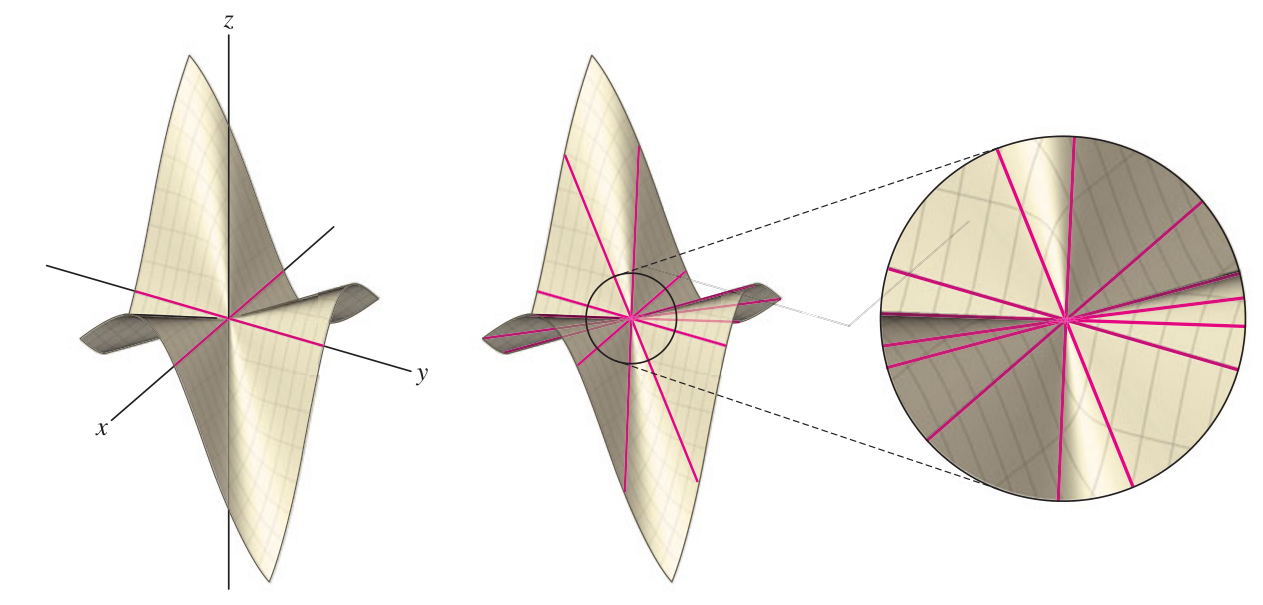
The concepts of continuity and differentiability are more complicated in 3d due to potential incompatibilities of directionality that are a function of the and relationship.

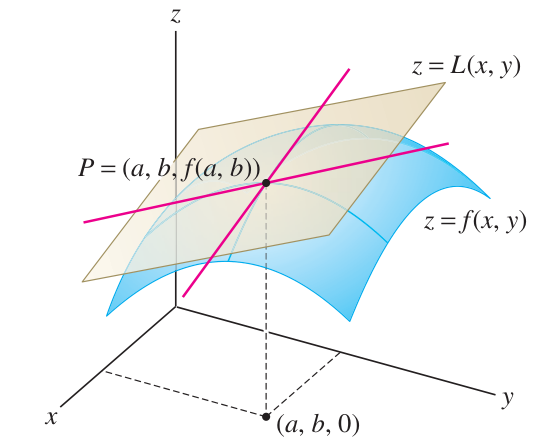
Linear approximation

There is a relation between the concepts of linear approximation, partial derivative, tangent plane, and differentiability. This relation is contained in a function defined in terms of :

Linear approximation function

The linear approximation function includes both partial derivatives and . The set of points satisfying defined by the above equation, namely the graph of , is the tangent plane. Lastly, the function is said to be differentiable when:

with two functions and satisfying as .

If is not differentiable, then the linear approximation may be a bad approximation.

Linear approximation in 2d

Remember that for a function of a single variable, we have the linear approximation:

The tangent line to at is given by , and is considered differentiable when such that as :

Tangent plane via tangent lines

How do we know that the graph of gives the tangent plane?

The tangent vector to the trace at is given by . So the tangent line is given by:

These points satisfy . The graph must be the tangent plane because it is the unique plane such that the tangent lines of the trace curves and lie in this plane.

Taylor series and linear approximation

Linear approximation gives the first two terms of the Taylor series of a function, and the remainder term, captured in , must limit to zero when the function is differentiable:

If agrees with its Taylor series, then:

Differentials

Some authors use the mnemonic notation of finite differentials for applications of linear approximation. These are written as , , , , etc., even though they are not infinitesimals. Their usage is according to the following kind of rules:

Example

Tangent plane to paraboloid

Problem: Find the equation of the plane tangent to the paraboloid at . Solution: Set . Compute , . So , , and the linear approximation is given by:

The tangent plane is found by setting .

Exercise 09B-01

Tangent plane to a graph

Let . Find the tangent plane to the graph of at the point .

Exercise 09B-02

Linear approximation

Use a linear approximation to estimate the value of .

• (a) Write this using a function .
• (b) Write this using the notation of differentials.

What is the percentage error of your estimate from the true value?

Differentiability

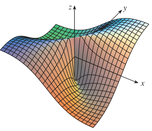
In 2d, a function is differentiable precisely where its derivative exists. The situation is not so simple in 3d: a function like has both partial derivatives at , but it is not differentiable there! On the other hand, one theorem does help:

Theorem

If a function is given and both partials and exist and are continuous at a point , then is differentiable at .

Exercise 09B-03

When partials aren’t continuous

Compute the partial derivatives of and explain carefully why this non-differentiable function does not violate the theorem.

Exercise 09B-04

Differentiability of the radius function

Let . Is differentiable? Where?

Differentiable, but partials aren’t continuous:

The function is differentiable at since it is approximated by its tangent plane at . The partials are not continuous there! You may check this by computing and . You can also compute , which is not continuous at .

Problems due 22 Oct 2023, 9:00pm

Problem 09-01

Partial derivatives

• (a) Find .
• (b) Find .
• (c) Compute for . (Hint: you can use a different order on each term!)
• (d) The Laplace Operator is defined by . It is very important! Show that and and are all annihilated (sent to 0) by .

Problem 09-02

Linear approximation

Use linear approximation to estimate the value of without a calculator, using the notation of differentials. Then compute the exact value on a calculator and find the percentage error.

Problem 09-03

Tangent planes

• (a) Find the tangent plane to the graph of at the point .
• (b) Suppose , and . Find an approximate equation of the tangent plane to the graph at the point .
• (c) Find out where the tangent plane to has normal vector . (Hint: by inspection of the equation , you can write a general formula for the normal vector to a tangent plane. Insert an arbitrary point and solve for and to be where this normal vector aligns with the given one.)

Problem 09-04

Please write up and submit exercises 09A-03, 09A-04, 09B-01, 09B-02, 09B-04.