Line integrals II: vector fields, aligned
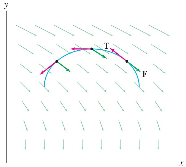
The aligned vector line integral is the integral of a vector field over a curve according to its alignment with the curve. It measures how much the vector field flows along the curve. It does not depend on the chosen parametrization (i.e. on the speed), but its sign depends on the direction traveled along the curve. It is given for a parametric curve that traverses its image one time, together with a vector field , by the formula:
Here we use the infinitesimal vector . This is the tangent vector scaled by ; alternatively it is the vector of infinitesimal travel of the particle during .
The same line integral is sometimes written with a different notation:
This notation is produced by writing and expanding the dot product.
To evaluate a line integral in this notation, first write a parametrization that traverses exactly once, then substitute for , and for , and for , then factor out the and evaluate the integral in .
Exercise 11A-01
Vector line integral over a curve
Compute the line integral , where and is traversed by the parametric curve , .
Example
Vector line integral
Problem: Compute , where is an ellipse parametrized by .
Solution: First calculate that and . Plug everything into the integrand to obtain:
Simplify this and evaluate:
Exercise 11A-02
Vector line integral over a segment
Compute the line integral , where is the line segment from to .
Optimization
Review of 1D theory
A regular point of a function is a point where . A critical point is a point where is either zero or undefined. In calculus, the theory of optimization (finding extremal values) is largely a theory of critical points.
Given a function of a single variable, its extrema occur either on boundary points of the region, or at critical points of in the interior of the region. For a closed interval , the boundary points are and , while the interior is the open interval . Every interior point is either regular or critical. To find extrema, therefore, it suffices to check boundary points, interior points of non-differentiability, and interior points where the derivative is zero.
All of this reasoning may be derived from the linear approximation:
Linear approximation:
If exists at , we can write near as:
Here , , and . Now rewrite this as . If , then for small enough, because as . This means there are points close to for which (with ), and points for which (with ). Conversely, if , there are points near for which and for which .
It follows that if is a regular point, meaning , then is certainly neither a local maximum nor minimum.
The critical points can be evaluated using the first and second derivative tests. For example, if the sign of crosses zero at from above, or if , the point is a local maximum.
2D theory
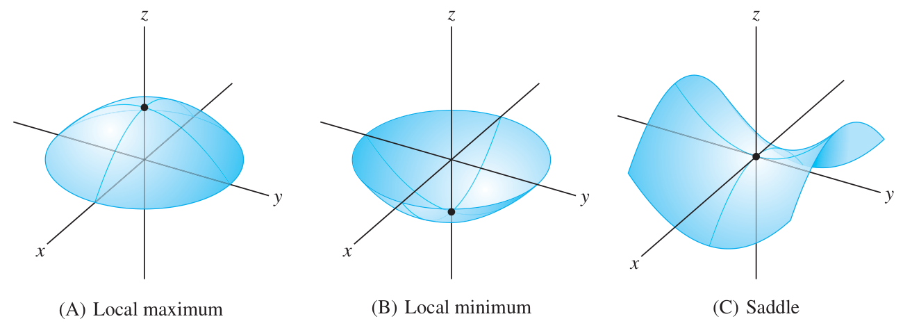
The 1D theory may be applied directly to the trace curves of a function , i.e. the curves given by or . The result is that if , or if , then is neither a local maximum nor minimum, but rather it would be possible to increase or decrease by moving along the respective trace curve.
A critical point of is a point such that either , or at least one of doesn’t exist. All extreme values of in the interior of a region must occur, therefore, at critical points.
(Note: the situation where, say, fails to exist while , counts as a critical point in these notes, but some other authors would not count it. Such points cannot be local extrema by the trace-curve reasoning applied to .)
The definition of critical points can be encapsulated in a single statement about the gradient:
Info
The point is a critical point of if and only if: or is undefined.
Global extrema are either local extrema (critical points in the interior), or they lie on the boundary. To check the boundary, one must find a parametrization of the boundary as a curve , and then optimize the scalar function of the single variable using the 1D theory. The extrema on the boundary should then be compared with the local extrema in the interior.
As in the 1D theory, critical points of can be either maxima or minima or neither, and there is a tool involving second-order partials that allows us to classify critical points in many cases. It is called the discriminant. Suppose that exist and are continuous near , a critical point of . Define the discriminant by the formula:
This formula is easy to remember as the determinant of the matrix of second-order partials:
Discriminant test
Let be a critical point near which the second-order partials are continuous.
- If the test is inconclusive
- If then is a saddle point
- If then is a max/min:
- If or then is a min
- If or then is a max
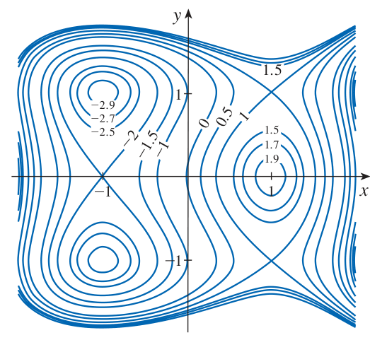
Exercise 11A-03
Classify critical points on topographical contour map
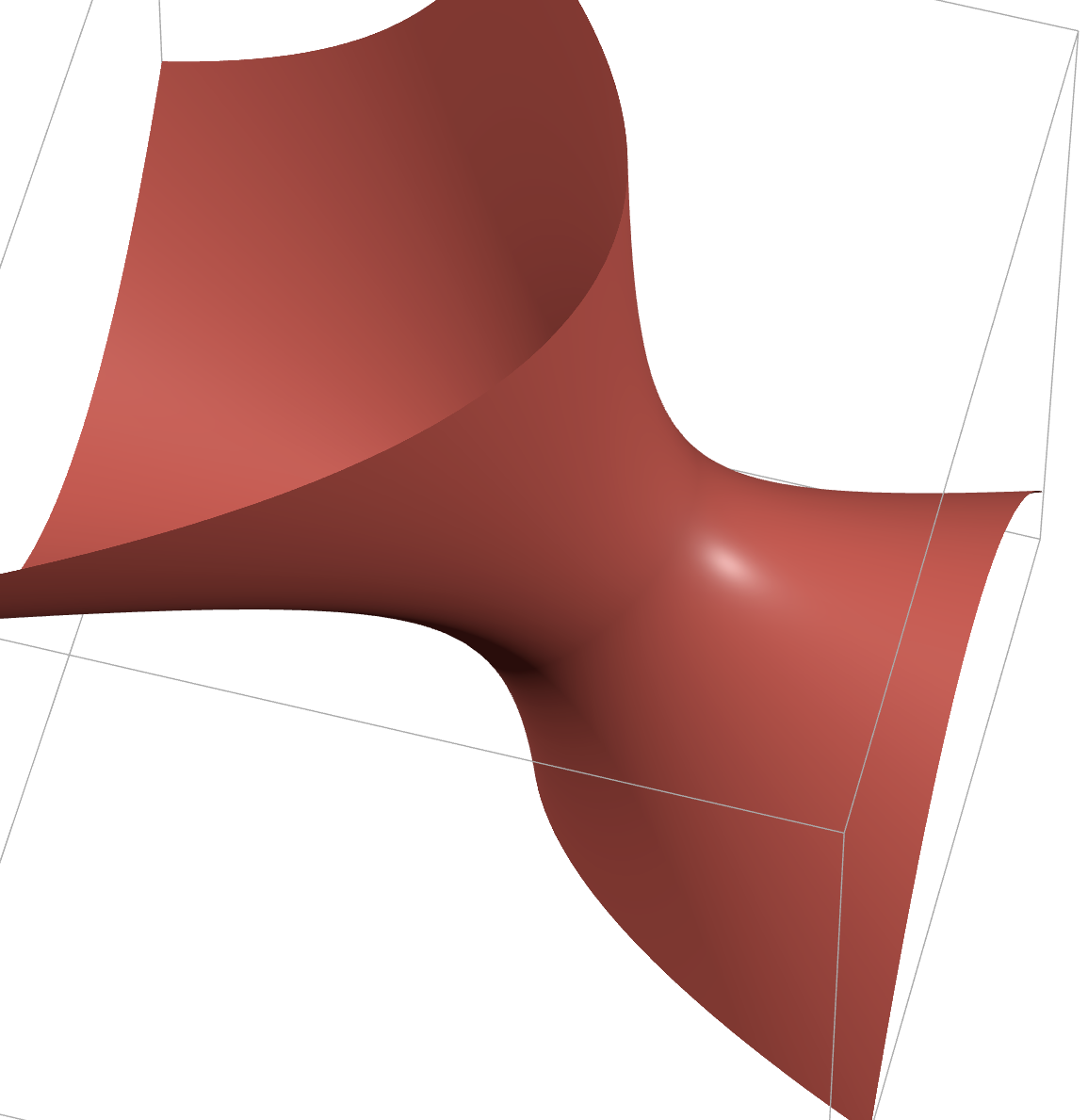
Example
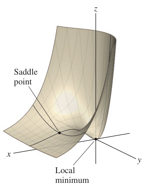
Minimum vs. saddle
Problem: Consider the function :
Determine the local extrema of by finding and analyzing its critical points.
Solution: We set and solve this system of equations for points . By computing the partials, we obtain:
The second equation implies because is never zero. Plugging this fact into the first equation gives which implies . So the critical points as given by components are and .
Now let us analyze these critical points using the discriminant. Compute:
Therefore , and in particular , . We also need and . The discriminant test concludes that is a local minimum, while is a saddle point.
3D plot: https://www.math3d.org/cDHxQockR
Also try Desmos3d: https://www.desmos.com/3d/17d5d68086
Exercise 11A-04
Analyze two critical points
Exercise 11B-01
Maximum on closed domain
Find the global maximum value of on the square , . Where does this occur? Remember to check critical points on the interior and optimize the function on the boundary.
Example
Minimal distance
Problem: Consider the surface given by points with coordinates satisfying . Find the point(s) closest to the origin.
Solution: Our goal is to extremize the distance to the origin of an arbitrary point on the surface. The distance formula gives . This function will be extremized at the same place(s) that the function is extremized because is monotone increasing for positive inputs. So we minimize instead. Next we write the distance as a function of just two variables. Using the surface equation to determine , we write . Then:
Setting these simultaneously to zero and solving gives , and is or . The distance at these points is 3.
Exercise 11B-02 = Problem 11-03
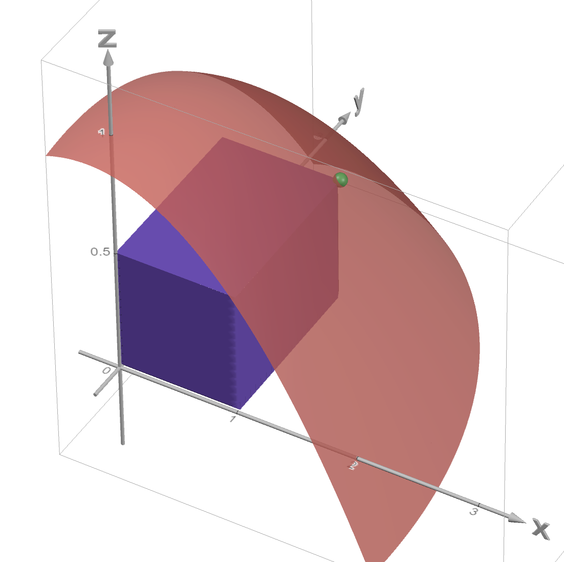
Biggest box
Find the largest volume of a box with nonnegative coordinates, all but one vertex on the coordinate planes, and the remaining vertex lying in the paraboloid given by . (So one corner is at the origin, and the opposite corner is on the paraboloid.) What are the dimensions of this box?
nD theory
(The technique for D requires knowledge of linear algebra, so the next discussion will not be tested in this course.)
In 3D, the same argument about trace curves shows that where is a non-zero vector, there is not a local extremum. At such a point, motion in the direction of will increase the value of , and motion in the (opposite) direction of will decrease the value of .
Similarly, in D one defines critical points as those points where is either or undefined. Local extrema of can only occur at critical points.
The matrix of second-order partials has a general form called the Hessian matrix:
In 3D the Hessian matrix looks like this:
In order to use to classify critical points, you have to compute its eigenvalues and count the number of positive and number of negative eigenvalues. (All positive minimum, all negative maximum, various signs saddle.) The determinant is the product of the eigenvalues, so in the 2D theory the discriminant reveals whether the eigenvalues have the same or opposite signs. This explains the discriminant rule that is used in 2D.
Constrained optimization: Lagrange multipliers
The setup is a function and a curve . The problem is to find the extremal values of on the curve. If the curve is given with a parametrization , then we could just extremize using the 1D theory. If the curve is instead given by a constraint such as , then there is another technique that can be much easier to implement than finding a parametrization for . It is called Lagrange multipliers. Since the constraint is written as , you can think of this as a relative of implicit differentiation.
The method of Lagrange multipliers makes use of the fact that when is extremized at on , then the gradients must align: for some scalar .
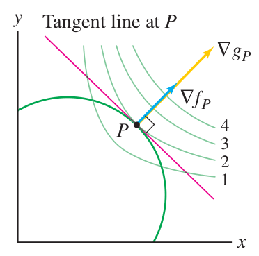
Gradients align at extremal values
The constraint curve is given as the level curve with . To show the gradients align, we show that they are both perpendicular to this level curve. Let be a parametrization of . We have already seen that:
for any , so is always perpendicular to the level curves. In addition, at the specific time where is extremized, we also have from the 1D optimization theory and the chain rule:
and this shows that is also perpendicular to the level curve at . Since both are perpendicular to the level curve, they must point along the same line.
Lagrange multipliers: parallel level curves
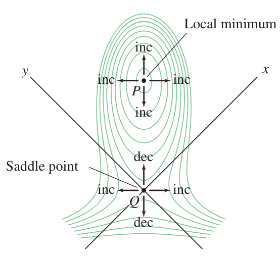
It is convenient to visualize the Lagrange condition on a contour map. The curve will be parallel to the level curves of at the points where the value of is extremized on .
If the level curves of are not parallel to at a point , then it is possible to increase or decrease by moving along because this motion will cross over level curves of .
Because is a level curve of , it is perpendicular to . So the level curves of and must be parallel at an extremal point. This happens if and only if the gradients are parallel.
Example
Lagrange multipliers
Problem: Find the extreme values of on the ellipsoid . Solution: We define . Write out the Lagrange Equations:
Solve the system of equations by first solving for in each coordinate and then equating these values:
Obtain and . Insert these expressions into the equation and find a single equation, the solutions of which are and . Using these expressions again, we find the other coordinates of two critical points:
Plug these points into and obtain and .
Since the ellipsoid has no boundary, these are the global max and min of on the ellipsoid.
Exercise 11B-03
Lagrange multipliers
Find the extreme values taken by the function on the curve that is given by the equation:
- (a) ,
- (b) ,
Problems due 6 Nov 2023, 10:00pm
Problem 11-01
Vector line integral
Compute , where and is the triangle with vertices , , (traversed in that order).
Problem 11-02
Study of critical points
Find the critical points of the following functions, and analyze them using the discriminant test (or state that the test fails). You may use a calculator or computer to evaluate the discriminant at the critical points.
- (a)
- (b)
- (c)
Problem 11-03
See above.
Problem 11-04
Additional exercises to write and submit: A-02, A-04, B-01, B-03.