Vector Calculus - Packet 13

In this packet we study a 2D version of the Fundamental Theorem of Calculus called Green’s Theorem. The 1D integral over the -axis is upgraded to a double integral over a 2D region . The derivative is replaced by a new kind of derivative called ‘curl’. The difference taken on the boundary of the 1D interval is upgraded to the line integral taken around the boundary of the 2D region .

Curl

Curl as derivative operator

Start with a vector field with vector components , where and are functions of points in space.

From this we create a scalar field called the scalar curl of , written . This field is calculated with the formula:

One way to remember this formula is to create a vector-derivative-operator with components , and then take the cross product “”, applying and to the function components of . (Interpret and as 3D vectors with zero -component.) The result is a vector with only a -component. The subscript indicates that we are just taking the scalar value of that -component.

Example

Computing scalar curl

Suppose . Then , considered as a function of .

Exercise 13A-01

Computing scalar curl

Compute , where .

Exercise 13A-02

Computing scalar curl

Compute , where .

Exercise 13A-03

Understanding curls

• (a) Draw the vector field .
• (b) Compute the curl , where .
• (b) Draw the vector field from 12A-02.

Exercise 13A-04

Line integral and vector field

What is the vector field being integrated in this line integral?

Curl as measure of circulation

The scalar curl field can be explained as a measure of circulation of the vector field around each point in space. 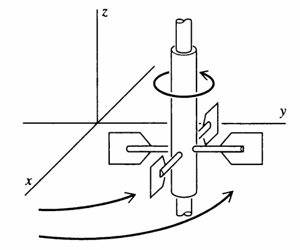It is good to understand how this works. Below we calculate the circulation of around a small box. In a Problem, you calculate the circulation of around a small circular loop.

Consider a small box with bottom left corner at a point in the plane, and sides of length and . Label the sides with subscripts for left, right, top, bottom as in the picture: 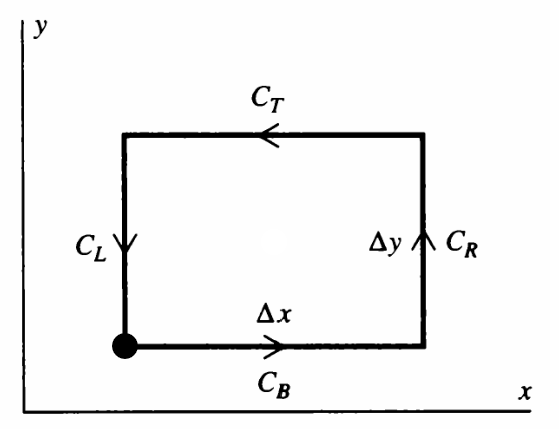The ‘circulation’ we wish to calculate is the aligned vector line integral around this box:

Break this into four integrals, one over each side of the box. Define parametric curves traversing each side, with for each case:

• For side , take .
  • Observe that and .
• For side , take .
  • Observe that and .
• For side , take .
  • Observe that and .
• For side , take .
  • Observe that and .

Notice that on , and the others simplify in a similar way because of the zeros in the vectors.

We are considering small boxes , and we will in fact take a limit as the sides go to zero. It is appropriate to use the linear approximation for each component and on the box, with differentials from the point . This lets us write the circulation integral in terms of and , evaluated at the point ; these appear in the curl formula we are trying to explain. Write for the components of .

• For side , we have .
• For side , we have .
• For side , we have .
• For side , we have .

Now plug everything in and compute four integrals in :

Simplify this by cancelling some terms and combining some others:

Notice that is the area of the box. The bigger the box, the greater the effect of circulation.

The scalar curl is the limit of the ratio of circulation to the enclosed area, for boxes shrinking to zero:

Exercise 13B-01 = Problem 13-02

Circulation calculated around circles

Repeat the reasoning above but going around a small circle instead of a box. You can use the single parametrization for a small constant, and the center point of the circle.

The derivation is faster with this method, but circles do not tile the plane the way boxes do, and we need a tiling of the plane to prove Green’s Theorem.

Green’s Theorem

The main theorem of 2D calculus is called Green’s Theorem, but it could be called more expressively “The Fundamental Theorem of 2D Calculus”. It says that the integral of curl over a region is equal to the total circulation on the boundary:

Green’s Theorem

When is a region of the -plane with boundary , then:

Writing this in terms of component functions, we have:

Example

Area of a region calculated from the boundary

Set . Then while , so the LHS of Green’s Theorem reduces to the enclosed area. We then have:

For example, an ellipse is given by . Note . The area of an ellipse is therefore:

Example

Faster calculation of line integral using Green’s Theorem

Problem: Find , where is given as in the picture: Solution: The interior of the region is covered by one double integral in polar coordinates, and that is easier to compute than four line integrals, so we use Green’s Theorem to convert to a double integral. We choose the vector field so that gives the line element. Then , and we compute:

Exercise 13B-02

Faster calculation of line integral using Green’s Theorem

Compute , where is the triangle with vertices , , and (traversed in order).

Understanding Green’s Theorem

To understand the reasoning behind Green’s Theorem, it is important to remember why the 1D version of the Fundamental Theorem of Calculus is true.

FTC derivation reminder: telescoping summation

Let . We would like to see why .

If and are very close, we could write . Ignoring the error term, we see that , and the RHS is the area of a box with base and height . This is when is very small.

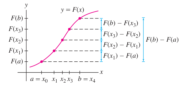
If and are farther apart, divide into intervals:

Assume for simplicity that for every . Now analyze each small difference using a linear approximation:

Subtracting from both sides and plugging into the summation, obtain:

If we ignore the error term and take the limit as with , then the first summation (a Riemann sum) becomes .

To account for the error term properly, take small enough that for some fixed positive number . Then as the error summation limits to zero:

To summarize, the key idea is that we add up all the small differences . In the sum, internal cancellation occurs, leaving just the boundary difference . On the other hand, each small difference is approximated by . (The linear approximation of using .) The sum of these terms is exactly the Riemann sum for the integral .

Even more briefly, the integral adds up many microscopic differences in which are written in the form .

Green’s Theorem can be explained with exactly the same process, except that instead of differences, we have circulations, and instead of that approximates a small difference, we have that approximates a small circulation. To add up circulations, we collect 2D squares, but there is still internal cancellation leaving only the terms on the boundary curve of the region.

Derivation of Green’s Theorem

We need to divide the region into microscopic squares. Let each square be identified by its bottom-left corner at point , where . Each square has width and height . Let denote the set of squares fully contained inside (specifically, the set of ordered pairs identifying the bottom-left corner of a square contained in ).

The circulation around the square at is approximated by . The error terms need to be collected as well; the exact circulation differs by an error term with magnitude less than , where is a positive function of satisfying , for some , as . (Notice that this can be chosen so it doesn’t depend on by taking the biggest one of those used for any of the squares in .)

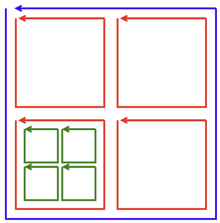
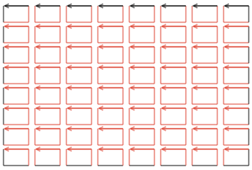
Now we add up all the circulations. The internal sides of boxes, which are shared between two boxes, will have a component of the integral traversed in each direction. These traversals contribute the same number with opposite signs, and therefore cancel. So, the total sum of circulations is equal to the circulation around the outer edges of the shape made by all squares of width which fit entirely in the domain. This is a 2D version of the cancellation in 1D that occurs between and , for example.

Considering now the sum of approximations, we have the sum of the values multiplied by the area of the squares, . This is a Riemann sum that limits to as and the number of boxes goes to . So the circulations add up to the boundary circulation around the squares contained in , and the sum of approximations using adds up to the integral of over the region.

Now let’s address the error term. Each small square has an error less than , which is less than for some positive number based on the guarantees on the behavior of . The number of boxes is . Let’s say the total area of the region is . The area covered by the boxes is so , and thus . The total error with all boxes is less than . But as . So the total error goes to zero.

Going deeper

One remaining issue should be addressed. Does the boundary converge to the boundary of ? Or, at least, does the circulation on the boundary of the collection of squares converge to the circulation on ?

This question is difficult to address using the concepts in this course. Instead of addressing it fully, we just explain how the circulation on a squared boundary can approximate the correct circulation on an angled boundary. Strictly speaking, this kind of explanation will then work for polygons, but by considering linear approximations of boundaries, the explanation is also good for smooth boundaries that have first derivatives.

Consider an angled line segment parametrized by for . Approximate this by rectangular stair steps, two vertical for every one horizontal, of width . Consider the bottom step , with horizontal piece and vertical piece . The line integral over this step, horizontal and vertical, is:

whereas the line integral over the corresponding segment of , written , is:

If we assume is small enough that is (nearly) constant on the square containing and , then these two values are nearly equal. One can then take the sums over all on one hand, and on the other hand, and track errors as before, and find that as they converge to the same thing.

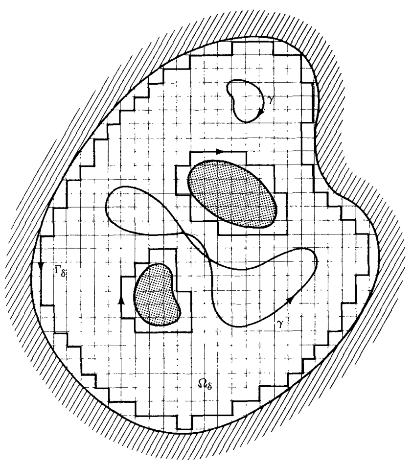
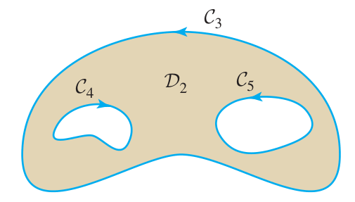
Interior boundary curves

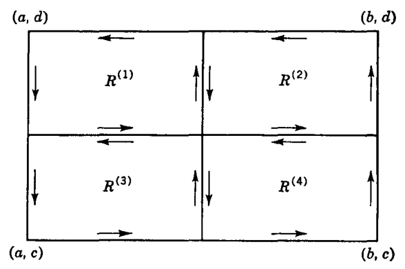
Some shapes have boundary lines on the inside. Do not forget to include these lines as part of the total boundary in Green’s Theorem! The orientation of these lines should be consistent with counter-clockwise circulation around infinitesimal boxes near the boundary. In the figure below, and are oriented correctly, while has the wrong orientation. The boundary is therefore .

Path dependence

Green’s Theorem expresses a relationship between circulation around the boundary and infinitesimal circulation in the interior. (Infinitesimal circulation is the curl times ). It says that adding up all the infinitesimal circulations gives the boundary circulation.

This relationship, considered from another angle, is connected to the idea of path independence. Consider two particle paths travelling between the same start and end points. Write for the first path, parametrized by , and for the second path, parametrized by . Write for the starting point, and for the ending point. 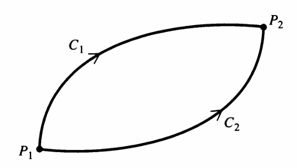Now consider the question: do the line integrals and have the same value for these two paths?

The vector field is said to be conservative or path independent if the answer is yes, and path dependent or non-conservative if the answer is no.

Consider the question more quantitatively. What is the value of the difference ? In fact, this difference is the same as the sum of line integrals around a closed loop starting and ending at . The complete path is written as : 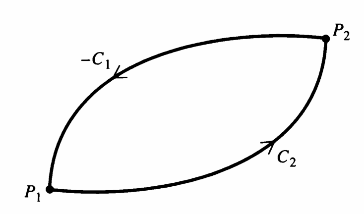(Here the path is the same path as but traversed in the opposite direction.)

By Green’s Theorem, the integral of over the region between the two paths gives the difference . In particular, if (in some region), then by Green’s Theorem the line integral from to does not depend at all on the path taken! (Provided the path remains in the region where .)

Path independence is also connected to the gradient:

Exercise 13B-03

Gradient fields are conservative

Suppose for some scalar field . Show that .

Challenge problem

(not for presentation)

Conservative fields are gradients

Suppose that . Find a scalar field such that . (Hint: define it using line integrals along paths!)

Simply connected regions

Path independence is equivalent to only for simply connected domains. These are domains without any holes, meaning that any loop can be tightened down to a point in the domain.

If there are holes, then it is possible to construct a field in the part of the domain outside the hole, such that there, but path independence is no longer strictly valid. Paths that wrap around the missing hole can have different line integrals. In fact, the line integral measures the number of times a path wraps around the hole. Two paths that wrap the same number of times differ by some enclosed region outside the hole where , so the line integrals on these paths must agree!

Exercise 13B-04

Gradient of angle

Let . Show that:

We saw above that for . Compute the integral , where is a path that winds -times around a circle of radius . (For example, with .)

Notice that is not defined at . So the applicable domain for Green’s Theorem has a ‘hole’ containing .

Problems

Problem 13-01

Biggest rectangle inscribed in ellipse

A rectangle is inscribed in the ellipse given by . The four points of this rectangle are given in coordinates by the four possibilities for . Using the method of Lagrange multipliers, find the largest possible area of such a rectangle in terms of the constants .

Problem 13-02

See above: Exercise 13B-01.

Problem 13-03

Shoelace Formula

Let give the components of a vector field in the plane. Observe that .

• (a) Let be a line segment from to . Show that:

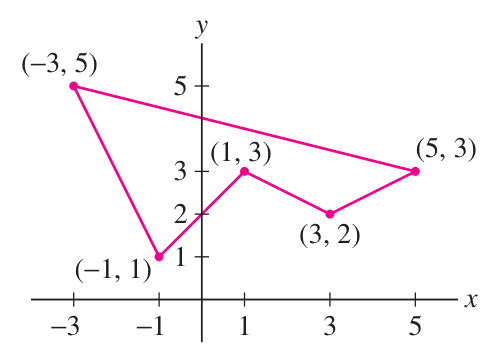
• (b) Let be the path traversing a polygon with vertices at , with , the edge segment connecting to . Show that the area of this polygon is given by:

• (c) Use the previous formula to find the area of this polygon:

Problem 13-04

Green’s Theorem Puzzle

Consider the following region and its boundary with circles of radius 1, 1, and 5: Suppose we know and . Suppose we know that on the tan region. Calculate .

Problem 13-05

Path independence

• (a) Show that the line integral does not depend on the path taken from to .
• (b) Find a function such that gives the vector field that is integrated in (a).

Problem 13-06

Submit exercises A-02, -03; B-01, -02, -04, ‘challenge problem’.