Fundamental Theorem of Line Integrals
The following conditions for a vector field are equivalent:
- is path independent,
- in the region (which is simply connected, i.e. no holes),
- for some scalar field .
When these conditions hold, is called conservative. Then for two paths and from to , and for a scalar field .
(Note: when the domain is not simply connected, then the curl condition is not strong enough, but the first and last conditions are still equivalent to each other and the word ‘conservative’ applies when these two conditions hold.)
The Fundamental Theorem of Line Integrals gives the value that is common to these line integrals over various paths:
FT of Line Integrals
For any path from point to point , we have:
If gives the elevation on a mountain at point , then gives the rate of incline in the direction of steepest ascent. The line integral of along any hiking path then gives the total change in elevation.
Derivation of FT of Line Integrals
Take any parametrization of given for . Now . By the chain rule for paths (in reverse), this is equal to . So can apply the ordinary FTC:
Exercise 14A-01
FT of Line Integrals: elevation gain
Consider the vector field . Choose any path between and . Verify the FT for line integrals by computing the elevation gain on your chosen path in two ways (computing both sides of the FT). For the right side, you will need to first find a field such that .
Line integrals III: vector fields, across
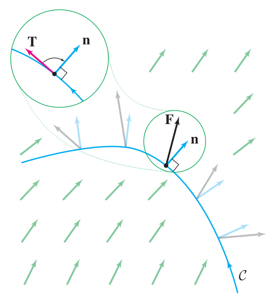
The across vector line integral is the integral of a vector field over a curve according to its alignment with the normal vector to the curve. It measures how much the vector field flows across the curve. It does not depend on the chosen parametrization (i.e. on the speed), but its sign depends on the direction traveled along the curve. It is given for a parametric curve that traverses its image one time, together with a vector field , by the formula:
Here is a scalar, and is after rotating clockwise by . If , then , and . Also .
The integrand is the scalar projection of onto the direction perpendicular to the curve at each point on that curve. (The positive direction means: rotate the orientation of clockwise by .)
The quantity computed by this line integral is sometimes called the flux across the curve.
This line integral is defined for curves in the plane, since the normal vector defined as a clockwise rotation of only makes sense for plane curves. (Rotation around the -axis.) In 3D, one computes the flux across a surface, and the “across vector line integral” is replaced by an “across vector surface integral”. On the other hand, the “aligned vector line integral” does make sense in 3D (or D).
Example
Vector line integral: flux across a path
Problem: Suppose . Compute the flux of across the curve for (oriented left to right). Solution: Use for . Then and . At , has the value . So , and .
Exercise 14A-02
Vector line integral: flux across a path
Let , and the line segment from to . Compute the flux of across .
Divergence
Divergence as a derivative operator
Start with a vector field with vector components , where and are functions of points in space.
From this we create a scalar field called the divergence of , written . This field is calculated with the formula:
One can remember this formula using the “vector” ; the formula expresses a dot product of and .
This formula naturally extends to higher dimensions. For example, in 3D we have:
Example
Divergence of vector fields
Consider the vector field . This is a radial field where each vector has length . everywhere.
Now consider the vector field . We have except at , where it is infinity (undefined).
In physics it is common to use polar (or cylindrical or spherical) coordinates because many problems have rotational symmetry. The derivative operators of vector calculus can be expressed in these coordinate systems.
Example
Divergence in polar coordinates
Let give a vector field in polar coordinates. Here and are scalar coordinate functions, is the unit vector in the radial direction, and is the unit vector in the direction. Problem: Find a formula for the divergence in polar coordinates.
Solution: Write in terms of polar coordinates. We have in Cartesian coordinates:
so:
The chain rule gives us formulas to convert derivatives:
So we obtain, after some cancellation and rearranging:
Polar divergence looks different
Given a vector field with polar coordinates and , its divergence is given by:
Exercise 14A-03
Polar divergence
Suppose are the Cartesian components for with some integer. Write this vector field using polar coordinates, and compute using the polar formula for divergence. Repeat the exercise with .
Divergence as measure of expansion
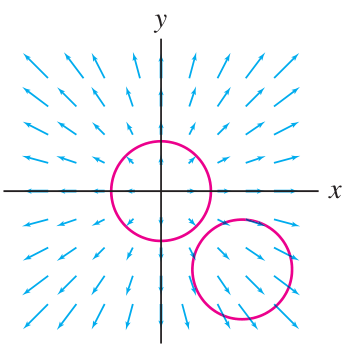
The divergence can be explained as a measure of expansion of the vector field at each point in space. (Negative divergence means contraction.) If the vector field corresponds to the velocity of a fluid flow, then divergence measures the rate at which fluid flows out of (or into) each point. We can verify this interpretation by using a vector line integral to measure the flow out of a circular loop, and then shrink the loop down to an infinitesimal loop.
Suppose is given. Let be a circle of radius centered at , oriented counter-clockwise. We will compute the vector line integral across in the limit as .
Calculate this integral using linear approximations for and . Let , and write and .
We have:
- ,
- where the partial derivatives are evaluated at .
Now and , so the line integral becomes:
In the limit as , this becomes , where is the infinitesimal area of the circle.
Divergence Theorem
The calculation showing that divergence measures flow out of a loop can be done for a box-shaped loop instead of a circle. When two boxes are glued side-by-side, flow out of one box and into the other contributes positively to the line integral around the first box, and negatively to the line integral around the second box, so these contributions cancel in the sum. By subdividing a region into infinitesimal boxes, writing for the total flow out of each box, summing the flow across all the box walls, and observing the inner cancellation of adjacent boxes, one obtains the divergence theorem:
Divergence Theorem
When is a region of the -plane enclosed by its boundary curve , then:
The way to think about this theorem is that measures local expansion of a fluid that is flowing with velocity vectors . Then measures the total expansion of fluid in the region . The theorem says that the total expansion in must exactly match the total egress of fluid from the region by flowing across the boundary . Net expansion exactly matches net outflow.
When in a region, then is said to be divergence free. An incompressible fluid flowing in a closed container is divergence free. This concept is the analogue of being conservative, with replaced by . Here is one mathematical application. For a divergence-free field, the flux between points and can be calculated using any path from to and does not depend on the chosen path. The reason is that any two paths create a loop, and the total flux across the loop is zero, so the flux into the loop on one side (the first path) equals the flux out of the loop on the other side (the second path). This is an analogue of path independence but for “across” line integrals instead of “aligned” line integrals.
Green’s theorem revisited
In 2D, it turns out that the divergence theorem and Green’s Theorem are actually restatements of the same fact about pairs of scalar functions.
Suppose . Then Green’s Theorem says that:
Now rotate the vector field clockwise by around each individual point , and call the new field . As we have seen with the components of , the components of are given by . Now the divergence of is the same as the curl of :
Furthermore, , so:
Putting this together, the two sides of the divergence theorem become:
So, in 2D, Green’s Theorem and the divergence theorem express the same relationship about the functions and on the region and its boundary . Green’s Theorem packages this relationship in terms of a vector field , and the divergence theorem packages this relationship in terms of the rotated vector field .
Problems
Problem 14-01
Faster calculation of line integral using divergence
Let be the box in the -plane defined by and . Let . Compute the line integral in two ways:
- (a) using separate line integrals over the four sides of the box,
- (b) using a double integral over the interior of the box.
Problem 14-02
Heat equation
Suppose the temperature in a region is given by the scalar field . Heat flows from hot to cold, following the negative temperature gradient .
The rate of total heat flow into a microscopic disk enclosed by the circle (radius , centered at ) is the vector integral of heat flow across the loop , namely: . Furthermore, the rate of change of is proportional to the net heat flow into (assuming is small enough).
Suppose that all temperatures are static in a region . (This doesn’t mean all temperatures are equal, since there could be a source or sink of heat on the boundary and a temperature gradient across .) This implies that the net heat flowing into and out of any disk fully contained within is zero.
Using the divergence theorem, explain why the temperature across must satisfy the partial differential equation . (Recall that the Laplacian operator applied to gives .)
Problem 14-03
Electric field: loop detector of contained charge
The planar electric field generated by a point charge at the point has the form:
Find the total electric flux exiting any given loop in the plane. Your answer should be one value for any loop that encloses the point , and another value for loops that do not.
For any loop that does not enclose , consider the value of in the region of the loop and apply the divergence theorem.
You cannot apply the divergence theorem to a region containing the point because is not defined at . So, for a loop that does enclose , you should first compute the answer directly for a small circular loop inside the given loop, and then apply the divergence theorem to the region enclosed between the larger given loop and your small circular loop.