Parametric surfaces
The 2D version of a parametric curve is known as a parametric surface. Two parameters are needed to control the two independent dimensions of the surface. Component functions give the coordinates for each pair of values :
Example
Common parametric surfaces
- (a) A vertical cylinder may be given parametrically by:
\mathbf{r}(\theta,z) = (R\cos(\theta),R\sin(\theta),z).
- (b) A sphere of radius $R$ may be parametrized by: ParseError: Can't use function '$' in math mode at position 26: …here of radius $̲R$ may be param…\mathbf{r}(\theta,\varphi) = (R\cos(\theta)\sin(\varphi),R\sin(\theta)\sin(\varphi),R\cos(\varphi)).
- (c) The graph of a function of two variables, $z=f(x,y)$, may be parametrized by: ParseError: Can't use function '$' in math mode at position 49: …two variables, $̲z=f(x,y)$, may …\mathbf{r}(u,v)=(u,v,f(u,v)).
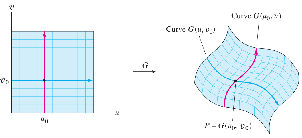 By holding constant or constant, one obtains grid curves. These correspond to trace curves when is the graph of a function, .
The two tangent vectors to the grid curves are computed by components, like the tangent vector of a parametric curve:
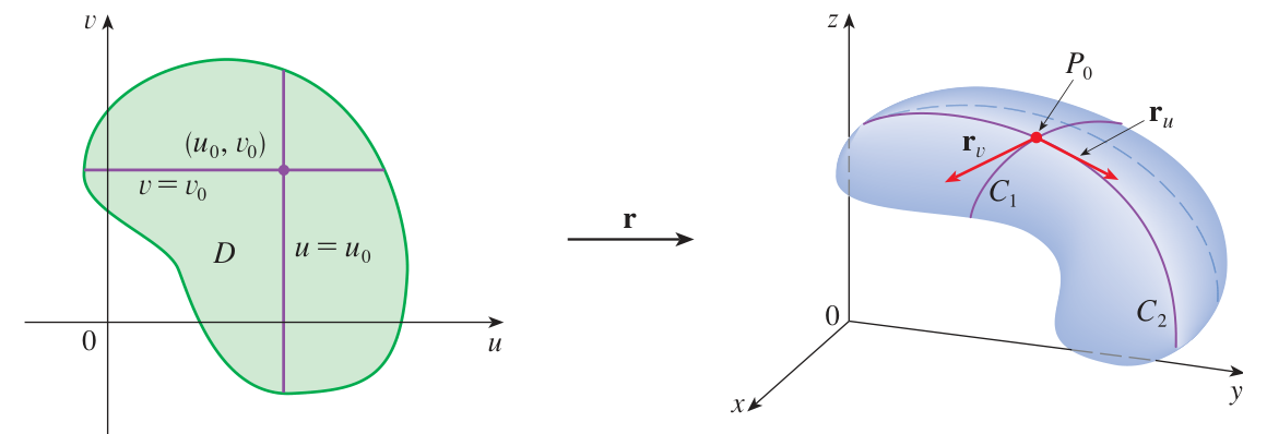
The tangent plane at a point on a surface given parametrically is given by taking all linear combinations of the tangent vectors added to the given starting point:
The cross product has several useful features:
- The direction of this cross product is normal to the tangent plane at the point . So the tangent plane could also be given in vector form by:
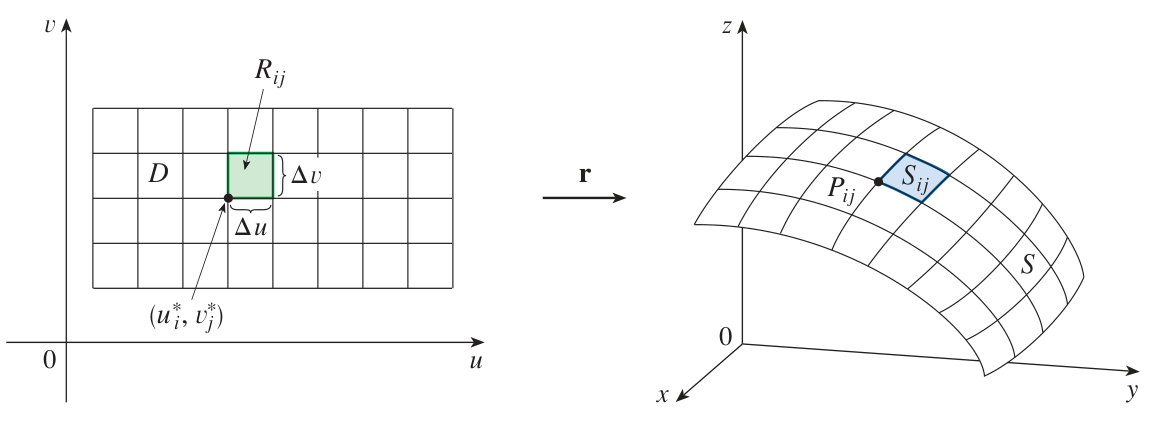
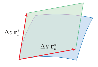
- The norm of this cross product gives a measure of area of the parallelogram created by and , so:
gives the area of a microscopic region on the surface that corresponds to the area in the parameter space . This formula is analogous to the formula used to calculate the arc length distance along a curve.
Example
Surface area
Problem: Find the approximate surface area of the surface given parametrically by:
where and . Solution: First, the tangent vectors are and . Their cross product is . The norm is . Compute the surface area by integrating :
Exercise 15A-01
Surface area of a torus
A circle in the -plane, offset on the -axis by from the origin, satisfies the equation . When this circle is rotated about the -axis, the result is a torus. To find the equation it satisfies, replace the variable with the radial quantity in the -plane:
This torus may be described parametrically by the formula:
Calculate the surface area of this torus. Your answer should be a simple expression in terms of and .
Exercise 15-02 = Problem 15-01
Theorem of Archimedes: band of a sphere
A band of a sphere is formed by taking the region of the sphere lying between two horizontal planes. Archimedes discovered that the area of a band of a sphere is equal to the area of the corresponding band of a cylinder that circumscribes the sphere. Prove this result. Use a sphere centered at the origin of radius , a vertical cylinder at the origin of radius , and horizontal planes given by and .
(Hint: you will need to solve for the range of azimuthal angles that corresponds to the range by using the last component function of the parametrization of the sphere.)
Change of variables
Recall that we can calculate iterated integrals of a function :
Such an integral can be interpreted as the volume (with sign) under the graph of .
Sometimes it is convenient to change variables before attempting to evaluate such an integral. This is a 2D analogue of -substitution. Oftentimes in 2D it is useful to change variables to simplify the bounds, not just to simplify the integrand. For example, sometimes one can express the region in terms of a rectangle in new coordinates, and compute the new integral as an iterated integral with constant bounds.
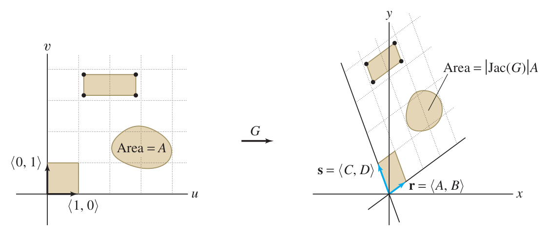
To change variables from to , first substitute functions and in place of and inside . Next, consider that parametrizes the -plane using the new variables . Then change the area element as follows:
Sign included
This formula is essentially the same as the one we used for , except that we include the sign that comes with , leaving out the absolute value.
This is the analogue of in -substitution, where if then . (Rather than , which would produce .)
Notice that the order matters: if we swapped the role of and , then would gain a minus sign. This is a novel feature of signs in 2D that relates to geometry via the right-hand rule.
In this situation, the item is also known as the Jacobian, or (when that name is used for the matrix itself), the Jacobian determinant:
Using this notation, we can rewrite the formula for change of variables:
Exercise 15A-03
New variables to improve the bounds
Let be the domain given by and . Change variables and then compute the integral:
(Hint: let and , so and .)
Surface integral: scalar
A scalar surface integral adds up the values of a function on a surface multiplied (locally) by elements of surface area on the surface. Given a surface in parametrized by (for with some domain in the parameter space that maps to ) and a scalar function , we can compute a surface integral of over with the formula:
This formula is the 2D analogue of the formula for a scalar line integral: .
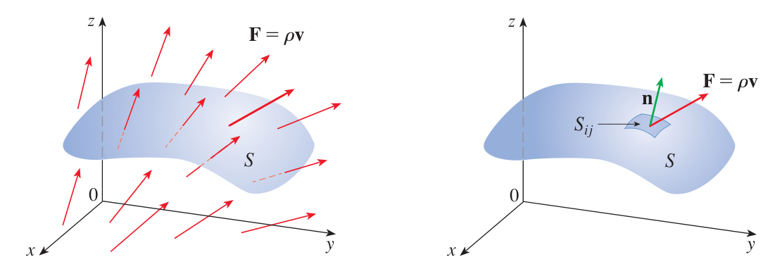
Surface integral: vector: flux across
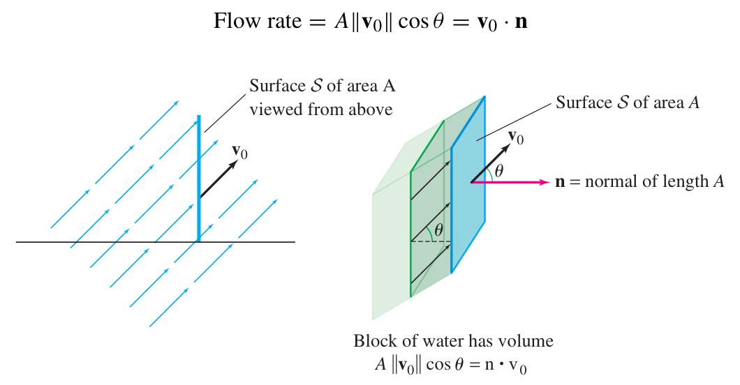
A vector surface integral adds up the total amount that a vector field crosses a surface . This total is called the flux across . When is the velocity vector field of a fluid flow, the flux quantifies the total rate of flow crossing the surface. It is defined like the ‘across’ line integral, but instead of derived from a rotation of the tangent vector , we use derived from the normal vector to the surface, . In terms of a parametrization of the surface , it is computed using the formula:
Here is a vector with length and direction , normal to the surface. So because . This is analogous to in the ‘across’ line integral.
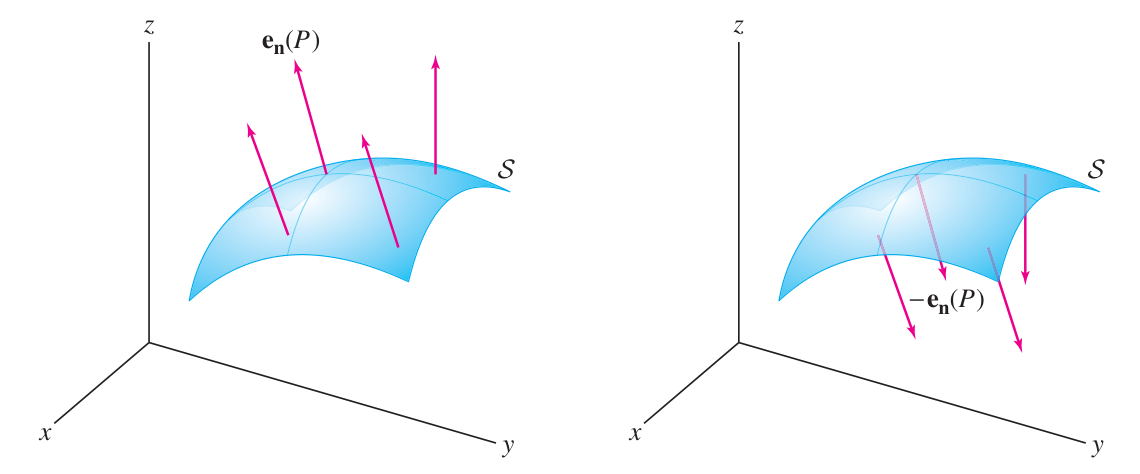
As with line integrals, the sign of the vector surface integral depends on the orientation of the surface. In 2D the orientation is the direction of . This direction comes from the cross product and thus it depends on the order of and , as well as the sign of each of them. (Exchanging and , or setting , switches the direction of .)
Example
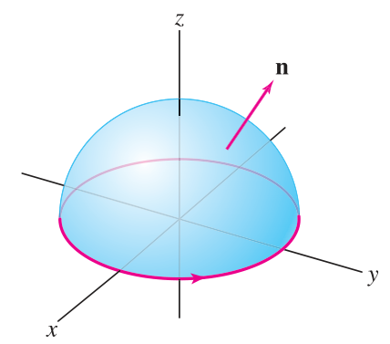
Upward flux through hemisphere
Problem: Let and let be the upper hemisphere of the unit sphere, oriented up and out. Compute the total flux of across .
Solution: First we need a parametrization of with the correct orientation. Try , and check the orientation after computing . For the upper hemisphere, the domain in the -space will be and . Compute:
Notice that is , which points inward, but the problem states that should be oriented with normal pointing outward, so we reverse the order, taking first and second.
Now plug into the vector field to find its values on the surface:
Then:
Finally we must evaluate the integral over the domain, using the fact that and :
Tip
Faraday’s Law of Induction states that the ‘aligned’ vector line integral of electric field around a curve is proportional to the rate of change of magnetic flux through the surface enclosed by :
Given a formula for the current flowing in the linear wire, one computes the magnetic field in the region above the linear wire. By integrating over , one obtains the total flux as a function of time; taking the (negative of the) derivative gives the quantities in the Faraday identity above. Because for the voltage , the value of the line integral on the LHS is actually the voltage drop around the wire (by the FT of Line Integrals).
Stokes’ Theorem in 3D
Vector curl
We define a vector version of the curl:
Each component of gives the circulation around a small circle in the plane of the other two components. This data combines the information of circulations in each coordinate plane into a single vector.
Exercise 15B-01
Linearity of curl operation
Show that .
The direction of is the direction of a normal vector to the plane of strongest rotation. The magnitude of is the strength of rotation in that plane. The right-hand rule applies: the direction of will point along the thumb when the fingers curl in the direction of strongest rotation.
Checking the interpretation
To check these claims, one would have to set up a calculation of the circulation in the plane perpendicular to an arbitrary vector . This would be very technical and tedious. An easier argument, the details of which we also omit, is to show first that the circulation in the plane perpendicular to a sum of vectors equals the sum of circulations in the planes perpendicular to and , respectively. It would follow that the circulation in the plane of is the dot product of with the curl. Then the final claim is established with the same argument that shows that a gradient vector points in the direction of steepest incline.
Exercise 15B-02
Conservative vector fields have no curl
Show that if for some scalar field , then everywhere.
Stokes’ Theorem
Given a surface with normal vector giving the orientation, apply the right-hand rule with thumb along to find the direction of local rotations on . Place this near a boundary point in to find the compatible orientation of the boundary.
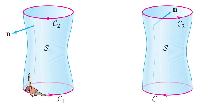
Stokes’ Theorem in 3D
For any surface with boundary (with compatible orientation), we have:
Exercise 15B-03 = Problem 15-02
Verify Stokes’ Theorem
Verify Stokes’ Theorem by computing the boundary line integral for the hemisphere example above, with .
Path independence
The arguments about conservative fields in the plane apply to conservative fields in 3D space. Instead of a region in the plane enclosed between two paths and , we use a surface in space that is bounded by the two paths and .
In any region in space, these conditions are equivalent:
- is path independent,
- for some scalar field .
These conditions imply the following condition:
- .
When the region in space is simply connected, the curl condition also implies the gradient and line integral conditions. If, conversely, the region has some holes in it, then it is possible for the first two conditions to fail even though the curl is zero everywhere (outside the holes).
Same curl? Differ by a gradient field.
When the region is simply connected, if two vector fields and have the same curl, i.e. , then they must differ by a gradient: for some scalar field . This is because , so for some .
Surface independence
We know that is path independent if and only if there is a scalar field such that . This fact about 1D paths can be upgraded to an analogous fact about 2D surfaces, with gradient replaced by curl:
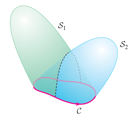
Surface independence for curl fields
Suppose the vector field arises as the curl of another field , so . Then for any two surfaces and which enclose the same boundary curve , the vector surface integrals agree (by Stokes’ Theorem), and can be computed as the line integral of around :
In this situation, the generating vector field is called the vector potential, by analogy to the scalar potential for a gradient field .
An important difference between and , though, is that must be constant when , while need not be constant in a region where .
The vector potential and the idea of surface independence play an important role in the theory of electromagnetism. One of the most famous phenomena in quantum physics, the Aharonov-Bohm Effect, involves a mystical connection between the mysterious vector potential of the magnetic field and an equally mysterious “complex phase” of the quantum wave function. (It is a mystical connection between mysterious entities because the traditional set-up of the physical theories suggests that the vector potential and the phase of the wave function are not physically real, but instead they’re arbitrary mathematical abstractions that partially describe the structures of the electric field and the quantum measurement probabilities, respectively.)
Divergence Theorem in 3D
We have already defined divergence in 3D:
The scalar field describes the rate of 3D expansion of at each point in space. One can show this by integrating a vector integral across a small sphere of radius , dividing by the volume of this sphere, and then taking the limit .
The divergence theorem relates the 3D integral of over the interior of a region of space to the vector surface integral of over the boundary of the same region:
Divergence theorem
For a 3D region with boundary , we have:
As for its 2D version, this theorem says that when the elements of local expansion times volume, quantified as , are added up across the full interior of , the result is equal to the total flux exiting across its boundary .
As before, to express the logic behind this theorem, one first divides the region into small cubes, adds the expansion elements for each cube, and takes the limit as the cube size goes to zero. Flux across an internal face of a cube corresponds to flux exiting one cube and simultaneously flux entering another cube, so internal cancellation occurs. Only flux exiting the boundary (crossing an external face) is not cancelled and thus contributes to the final result.
Example
Triple integral can be easier than six flux integrals
Problem: A box is given by . Calculate the total flux leaving this box for the vector field .
Solution: Instead of computing the vector surface integral for all six sides of the box, we compute the triple integral over the interior of the box. This equals the desired flux by the divergence theorem.
First find the divergence:
Now integrate for the answer:
Problems due 10 Dec 2023, 10:00pm
Problem 15-01
See Exercise 15A-02 above.
Problem 15-02
See Exercise 15B-03 above.
Problem 15-03
Curves wrapping around a cylinder
A vertical cylinder is given with axis the -axis. You do not know the radius.
Let . Suppose and are two simple curves wrapping one time clockwise around the cylinder. Show that:
Problem 15-04
Verify the divergence theorem
Verify the divergence theorem (by computing both sides and showing they agree) for the following data: and is the solid cylinder around the -axis with radius 2, height 5, and base lying in the -plane.