W03 Notes

Partial fractions

Videos

Review Videos

Videos, Math Dr. Bob:

• Partial Fractions 01 - Distinct Linear Factors
• Partial Fractions 02 - Repeated Linear Factors
• Partial Fractions 03 - Distinct Mixed Factors
• Partial Fractions 04 - Repeated Quadratic Factors
• Partial Fractions 05 - Composition with $e^x$

Link to original

01 Theory

Theory 1

A rational function is a ratio of polynomials, for example:

$$\frac{P(x)}{Q(x)}=\frac{5x^2+x-28}{x^3-4x^2+x+6}$$

Partial fraction decomposition

The partial fraction decomposition of a rational function is a way of writing it as a sum of simple terms, like this:

$$\frac{3x^3-5x^2-6x+20}{x^4-3x^3+4x}=-\frac{2}{x+1}+\frac{2}{{(x-2)}^2}+\frac{5}{x}$$

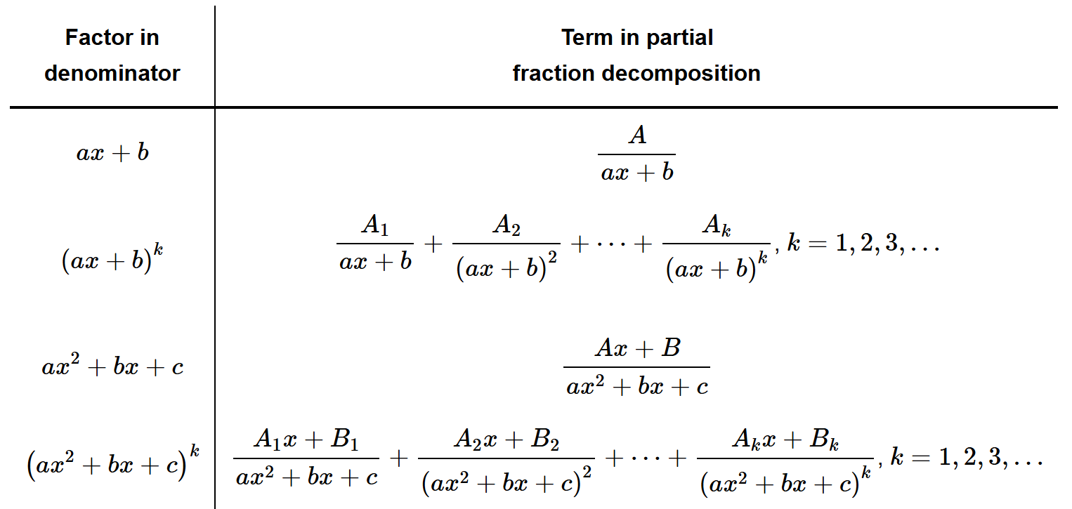
Allowed denominators:

• Linear, e.g. $x-a$, or linear power, e.g. ${(x-a)}^n$
• Quadratic, e.g. $x^2+bx+c$, or quadratic power, e.g. ${(x^2+bx+c)}^n$
  • Condition: quadratics must be irreducible. (No roots, i.e. $b^2<4c$.)

Allowed numerators: constant (over linear power) or linear (over quadratic power)

These are allowed as simple terms in partial fraction decompositions:

$$\frac{1}{x^2+1},\frac{2x+1}{x^2+5},\frac{7}{5x-8},\frac{1}{x},\frac{1}{x^3}$$

These are not allowed:

$$\frac{x}{x-1},\frac{x^3+2}{x^2+1},\frac{1}{x^2-1},\frac{1}{x(x-1)}$$

These are allowed, showing irreducible quadratic and higher powers:

$$\frac{x}{x^2+1},\frac{x^3+2x+1}{{(x^2+2)}^2}$$

In this example the numerator is linear and the denominator is quadratic and irreducible.

To create a partial fraction decomposition, follow these steps:

1. Check denominator degree is higher
   • Else do long division
2. Factor denominator completely (even using irrational roots)
3. Write the generic sum of partial fraction terms with their constants

Repeated factors – special treatment – incrementing powers

4. Solve for constants

Link to original

02 Illustration

Partial fractions with repeated factor

Partial fractions with repeated factor

Find the partial fraction decomposition:

$$\frac{3x-9}{x^3+3x^2-4}$$

Solution

(1) Check that denominator degree is lower. $✓$

---

(2) Factor denominator:

Rational Roots Theorem: check for roots at $\pm 1$ and $\pm 2$ and $\pm 4$.

Discover that $x=+1$ is a root. Therefore divide by $x-1$:

$$\frac{x^3+3x^2-4}{x-1}\gg \gg x^2+4x+4$$

Factor again:

$$x^2+4x+4\gg \gg {(x+2)}^2$$

Final factored form:

$$x^3+3x^2-4=(x-1){(x+2)}^2$$

---

(3) Write the generic PFD:

$$\frac{3x-9}{(x-1){(x+2)}^2}=\frac{A}{x-1}+\frac{B}{x+2}+\frac{C}{{(x+2)}^2}$$

---

(4) Solve for $A$, $B$, and $C$:

Multiply across by the common denominator:

$$3x-9=A{(x+2)}^2+B(x-1)(x+2)+C(x-1)$$

For $A$, set $x=1$, obtain:

$$\begin{array}{cccc}& & 3\cdot 1-9& =A{(1+2)}^2+B\cdot 0+C\cdot 0\\ \gg \gg & & -6& =9A\\ \gg \gg & & A& =-2/3\end{array}$$

For $C$, set $x=-2$, obtain:

$$\begin{array}{cccc}& & 3\cdot (-2)-9& =A\cdot 0+B\cdot 0+C\cdot (-3)\\ \gg \gg & & -15& =-3C\\ \gg \gg & & C& =5\end{array}$$

For $B$, insert prior results and solve.

Plug in $A$ and $C$:

$$3x-9=-\frac{2}{3}{(x+2)}^2+B(x-1)(x+2)+5(x-1)$$

Now plug in another convenient $x$, say $x=3$:

$$\begin{array}{cc}0& =-\frac{2}{3}\cdot 5^2+B\cdot 2\cdot 5+5\cdot 2\\ \frac{50}{3}-10& =10B\gg \gg B=\frac{2}{3}\end{array}$$

---

(4) Plug in $A$, $B$, $C$ for the final answer:

$$\frac{3x-9}{x^3+3x^2-4}=\frac{-2/3}{x-1}+\frac{2/3}{x+2}+\frac{5}{{(x+2)}^2}$$ Link to original

03 Theory

Theory 2

Partial fractions can be integrated using just a few techniques. Consider these terms:

$$\begin{array}{c}\frac{A}{x-a},\frac{A}{{(x-a)}^2},\frac{A}{{(x-a)}^3},\dots ,\\ \\ \text{and}\frac{A}{x^2+h^2},\text{and}\frac{Ax+B}{x^2+h^2}\end{array}$$

Linear power bottom

In order to integrate terms like this:

$$\frac{A}{{(x-a)}^n}$$

If $n=1$ then use log:

$$\int \frac{A}{x-a}dx=A\ln |x-a|+C$$

If $n>1$ then use power rule:

$$\int \frac{A}{{(x-a)}^n}dx\gg \gg \int A{(x-a)}^{-n}dx\gg \gg A\frac{{(x-a)}^{-n+1}}{-n+1}+C$$

Quadratic bottom, constant top

Formula for simple irreducible quadratics:

$$\int \frac{dx}{x^2+h^2}=\frac{1}{h}{\tan }^{-1}\left(\frac{x}{h}\right)+C$$

Memorize this formula!

Quadratic bottom, linear top

In order to integrate terms like this:

$$\frac{Ax+B}{x^2+h^2}$$

Break into separate terms:

$$\frac{Ax+B}{x^2+h^2}\gg \gg \frac{Ax}{x^2+h^2}+\frac{B}{x^2+h^2}$$

Then:

• First term with $x$ in top:

$$\int \frac{Ax}{x^2+h^2}dx\gg \gg \frac{A}{2}\ln |x^2+h^2|+C$$

• Second term lacking $x$ in top:

$$\int \frac{B}{x^2+h^2}dx\gg \gg \frac{B}{h}{\tan }^{-1}\left(\frac{x}{h}\right)+C$$

Extra - Completing the square when “no real roots”

To integrate terms with more general quadratics, like this:

$$\frac{A}{x^2+bx+c}$$

we need $b^2-4c<0$, i.e. “no real roots” of the quadratic. If that holds, then we can complete the square and substitute $u=\tan \theta$ as follows.

Look what happens when completing the square:

$$x^2+bx+c\gg \gg {(x+\frac{b}{2})}^2-\frac{b^2}{4}+c$$

Notice that $b^2-4c<0$ is equivalent to the condition $-\frac{b^2}{4}+c>0$. Create a new label $Z=-\frac{b^2}{4}+c$. So this condition means $Z>0$ and we can safely define $\sqrt{Z}$.

Then a $u$-substitution $u=x+\frac{b}{2}$ simplifies the equation like this:

$$x^2+bx+c\gg \gg u^2+{\sqrt{Z}}^2$$

The quadratic formula $x=\frac{-b\pm \sqrt{b^2-4ac}}{2a}$ shows that the condition $b^2-4c<0$ is equivalent to the condition “no real roots.” (In our case $a=1$. If we had $a\ne 1$, we could divide out this $a$ and change the others.)

So we see that “no real roots” is equivalent to the condition that the denominator can be converted to the format $x^2+h^2$ with some constant $h$.

At this point, to compute the integral, do trig sub with $u=\sqrt{Z}\tan \theta$ and $du=\sqrt{Z}{\sec }^2\theta d\theta$:

$$\begin{array}{c}\int \frac{Adx}{x^2+bx+c}\gg \gg \int \frac{A\sqrt{Z}{\sec }^2\theta d\theta }{Z{\sec }^2\theta }\\ \\ \gg \gg \frac{A}{\sqrt{Z}}\int d\theta \gg \gg \frac{A}{\sqrt{Z}}\theta +C\\ \\ \gg \gg \frac{A}{\sqrt{Z}}{\tan }^{-1}\left(\frac{x+b/2}{\sqrt{Z}}\right)+C\end{array}$$

Link to original

04 Illustration

Example - Repeated quadratic, linear tops

Partial fractions - repeated quadratic, linear tops

Compute the integral:

$$\int \frac{x^3+1}{{(x^2+4)}^2}dx$$

Solution

(1) Partial fraction decomposition:

• Numerator degree is lower than denominator.
• Factor denominator completely. (No real roots.)

Write generic PFD:

$$\frac{x^3+1}{{(x^2+4)}^2}=\frac{Ax+B}{x^2+4}+\frac{Cx+D}{{(x^2+4)}^2}$$

• Notice: repeated factor: use incrementing powers up to 2.
• Notice: linear over quadratic.

Common denominators and solve:

$$\begin{array}{c}{x}^3+1=(Ax+B)(x^2+4)+Cx+D\\ \\ \gg \gg x^3+1=A{x}^3+B{x}^2+(4A+C)x+4B+D\\ \\ \gg \gg A=1,B=0\\ \\ \gg \gg C=-4,D=1\end{array}$$

Therefore:

$$\frac{x^3+1}{{(x^2+4)}^2}=\frac{x}{x^2+4}+\frac{-4x+1}{{(x^2+4)}^2}$$

---

(2) Integrate:

Integrate the first term using substitution $u=x^2+4$:

$$\begin{array}{c}\int \frac{x}{x^2+4}dx{\gg \gg }^{u=x^2+4}\frac{1}{2}\int \frac{du}{u}\\ \\ \gg \gg \frac{1}{2}\ln |u|+C\gg \gg \frac{1}{2}\ln |x^2+4|+C\end{array}$$

Break up the second term:

$$\frac{-4x+1}{{(x^2+4)}^2}\gg \gg \frac{-4x}{{(x^2+4)}^2}+\frac{1}{{(x^2+4)}^2}$$

Integrate the first term of RHS:

$$\begin{array}{c}\int \frac{-4x}{{(x^2+4)}^2}dx\gg \gg -2\int \frac{du}{u^2}\\ \\ \gg \gg \frac{2}{u}+C\gg \gg \frac{2}{x^2+4}+C\end{array}$$

Integrate the second term of RHS using $x=2\tan \theta$:

$$\begin{array}{c}\int \frac{dx}{(x^2+4{)}^2}\gg \gg \int \frac{2{\sec }^2\theta d\theta }{16{\sec }^4\theta }\\ \\ \gg \gg \frac{1}{8}\int {\cos }^2\theta d\theta \\ \\ \gg \gg \frac{1}{8}\int \frac{1}{2}(1+\cos (2\theta ))d\theta \\ \\ \gg \gg \frac{1}{16}\theta +\frac{1}{32}\sin (2\theta )+C\\ \\ \gg \gg \frac{1}{16}{\tan }^{-1}\left(\frac{x}{2}\right)+\frac{1}{32}2\sin \theta \cos \theta +C\\ \\ \gg \gg \frac{1}{16}{\tan }^{-1}\left(\frac{x}{2}\right)+\frac{1}{32}2\frac{x}{\sqrt{x^2+2^2}}\frac{2}{\sqrt{x^2+2^2}}+C\\ \\ \gg \gg \frac{1}{16}{\tan }^{-1}\left(\frac{x}{2}\right)+\frac{1}{8}\frac{x}{x^2+2^2}+C\end{array}$$Link to original

Extra - “Rationalize a quotient” - convert into PFD

Extra - “Rationalize a quotient” - convert into PFD

Sometimes an integrand may be converted to a rational function using a substitution.

Consider this integral:

$$\int \frac{\sqrt{x+4}}{x}dx$$

Set $u=\sqrt{x+4}$, so $x=u^2-4$ and $dx=2udu$:

$$\gg \gg \int \frac{2udu}{u^2-4}$$

Now this rational function has a partial fraction decomposition:

$$\frac{2u}{u^2-4}\gg \gg \frac{2u}{(u-2)(u+2)}\gg \gg \frac{1}{u-2}+\frac{1}{u+2}$$

It is easy to integrate from there!

Practice exercises:

• To compute $\int \frac{\sqrt{x}}{x-1}dx$, try the substitution $u=\sqrt{x}$.
• To compute $\int \frac{dx}{\sqrt[2]{x}-\sqrt[3]{x}}$, try the substitution $u=\sqrt[6]{x}$.
• To compute $\int \frac{1}{x-\sqrt{x+2}}dx$, try the substitution $u=\sqrt{x+2}$.

Link to original

Simpson’s Rule

Videos

Review Videos

Videos, Math Dr. Bob:

• Simpson’s Rule with Error Bound

Videos, Organic Chemistry Tutor:

• Midpoint Rule and Riemans Sums
• Simpson’s Rule and Numerical Integration

Link to original

05 Theory - review

Theory 1

The Trapezoid Rule is a technique to approximate the area under a curve as the sum of areas of thin trapezoids whose top corners lie on the curve.

The tops of the trapezoids are lines that approximate the curve. They are determined as lines that agree with the curve at two points.

Trapezoid rule - area formula

Given a function $f$ and a partition of the range $[a,b]$ labeled by $x_0,x_1,\dots ,x_n$ (with $x_0=a$ and $x_n=b$), the Trapezoid Rule determines the area formula:

$$T_n=\frac{1}{2}\mathrm{\Delta }x(y_0+2y_1+2y_2+\cdots +2y_{n-1}+y_n)$$

Notice the pattern in $2$s and see how this formula comes about: The area of one trapezoid is $\mathrm{\Delta }x\left(\frac{y_{j-1}+y_j}{2}\right)$. All vertical values $y_1,\dots ,y_{n-1}$ (excepting the endpoints $f(a)$ and $f(b)$) are represented in two trapezoids, so their contribution is doubled.

Extra - Trapezoid rule - error bound

The error of the Trapezoid Rule approximation is bounded by this formula:

$$\mathrm{Error}(T_n)\le \frac{K_2{(b-a)}^3}{12n^2}$$

Here $K_2$ is any number satisfying $K_2\ge |f^{\prime \prime }(x)|$ for $x\in [a,b]$.

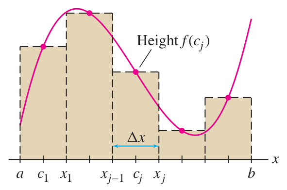
The Midpoint Rule is a technique to approximate the area under a curve as the sum of areas of thin rectangles whose top midpoints lies on the curve.

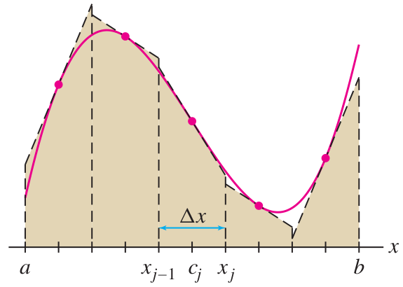
The very same formula also represents the areas of trapezoids whose top midpoints lie on the curve and whose top line is tangent to the curve:

The reason they are equal is simple: when pivoting the top line on the ‘attached’ midpoint, the area of the trapezoid does not change.

Midpoint Rule - area formula

Given a function $f$ and a partition of the range $[a,b]$ labeled by $x_0,x_1,\dots ,x_n$ (with $x_0=a$ and $x_n=b$), the Midpoint Rule determines the area formula:

$$M_n=\mathrm{\Delta }x(f(c_1)+f(c_2)+\cdots +f(c_{n-1})+f(c_n))$$

Here each $c_i$ is the midpoint of the interval $[x_{i-1},x_i]$. It can be given by the formula $c_i=a+(i-1/2)\mathrm{\Delta }x$.

Extra - Midpoint Rule - error bound

The error of the Midpoint Rule approximation is bounded by this formula:

$$\mathrm{Error}(M_n)\le \frac{K_2{(b-a)}^3}{24n^2}$$

Here $K_2$ is any number satisfying $K_2\ge |f^{\prime \prime }(x)|$ for $x\in [a,b]$.

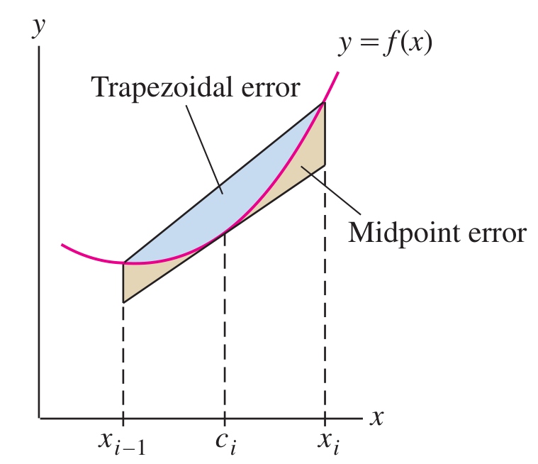
Notice that $M_n$ has an error bound that is $1/2$ of the bound for $T_n$. This does not mean that $M_n$ always has a smaller error than $T_n$. It means that without calculating the error, simply plugging numbers into the error bound formulas, we obtain a smaller bound for $M_n$ than for $T_n$. This is about our knowledge of the error, not the reality of the error.

Link to original

06 Theory

Theory 2

It turns out that the Midpoint Rule and the Trapezoid Rule tend to differ from the exact integral in opposite directions, and the Midpoint Rule tends to be twice as accurate. Therefore we may improve on both of them by constructing a weighted average of the formulas. This is called Simpson’s Rule.

Simpson’s Rule - defining formula

Simpson’s Rule is given by the weighted sum of the Trapezoid and Midpoint Rules:

$$S_n=\frac{1}{2}{T}_n+\frac{2}{3}{M}_n$$

Simpson’s Rule - computing formula

Given a function $f$ and a partition of the range $[a,b]$ labeled by $x_0,x_1,\dots ,x_n$ (with $x_0=a$ and $x_n=b$), Simpson’s Rule determines the area formula:

$$S_n=\frac{1}{3}\mathrm{\Delta }x(y_0+4y_1+2y_2+4y_3+2y_4+\cdots +2y_{n-2}+4y_{n-1}+y_n)$$

Simpson’s Coefficient Pattern

Memorize the pattern for Simpson’s Rule:

$$1,4,2,4,2,4,2,\dots ,1$$

Simpson’s Rule - error bound

The error of Simpson’s Rule approximation is bounded by this formula:

$$\mathrm{Error}(S_n)\le \frac{K_4{(b-a)}^5}{180n^4}$$

Here $K_4$ is any number satisfying $K_4\ge |f^{(4)}(x)|$ for $x\in [a,b]$.

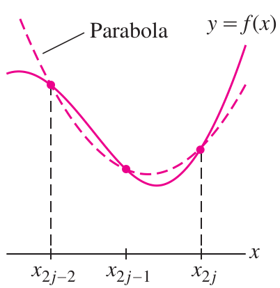
Simpson’s Rule $=$ “Parabola Rule”

The formula of Simpson’s Rule can also be explained or defined geometrically: it is the formula giving the sum of areas under small parabolas that meet the curve in three points.

There is a unique parabola passing through any three points with differing $x$-values:

These may be pieced together to form an approximation to the curve: The area under the parabola through $P_0$, $P_1$, and $P_2$ is given by this formula:

$$\frac{h}{3}(y_0+4y_1+y_2)$$

This formula may be verified using basic calculus (area under a parabola) and a lot of algebra. (Ambitious students should derive it.)

The area under the parabola through $P_2$, $P_3$, and $P_4$ is given by a similar formula:

$$\frac{h}{3}(y_2+4y_3+y_4)$$

The Simpson’s Rule formula is the sum of all these formulas! So the $2$s in Simpson’s come from duplication of endpoint terms as the “rectangular” regions are stacked end-to-end.

Link to original

07 Illustration

Example - Simpson’s Rule on the Gaussian Distribution

Simpson’s Rule on the Gaussian distribution

The function $e^{x^2}$ is very important for probability and statistics, but it cannot be integrated analytically.

Apply Simpson’s Rule to approximate the integral:

$${\int }_0^1{e}^{x^2}dx$$

with $\mathrm{\Delta }x=0.1$ and $n=10$. What error bound is guaranteed for this approximation?

Solution

(1) We need a table of values of $x_i$ and $y_i=f(x_i)$:

$x_i:$	$0.0$	$0.1$	$0.2$	$0.3$	$0.4$	$0.5$	$0.6$	$0.7$	$0.8$	$0.9$	$1.0$
$f(x_i):$	$e^{{0.0}^2}$	$e^{{0.1}^2}$	$e^{{0.2}^2}$	$e^{{0.3}^2}$	$e^{{0.4}^2}$	$e^{{0.5}^2}$	$e^{{0.6}^2}$	$e^{{0.7}^2}$	$e^{{0.8}^2}$	$e^{{0.9}^2}$	$e^{{1.0}^2}$
$\approx$	$1.000$	$1.010$	$1.041$	$1.094$	$1.174$	$1.284$	$1.433$	$1.632$	$1.896$	$2.248$	$2.718$

These can be plugged into the Simpson Rule formula to obtain our desired approximation:

$$\begin{array}{c}{S}_{10}=\frac{1}{3}\cdot 0.1\cdot (1.000+4\cdot 1.010+2\cdot 1.041+4\cdot 1.094+\cdots +2\cdot 1.896+4\cdot 2.248+2.718)\\ \\ \approx 1.463\end{array}$$

To find the error bound we need to find the smallest number we can manage for $K_4$.

Take four derivatives and simplify:

$$f^{(4)}(x)=(12+48x^2+16x^4)e^{x^2}$$

On the interval $x\in [\mathrm{0,1}]$, this function is maximized at $x=1$. Use that for the optimal $K_4$:

$$f^{(4)}(1.000)=206.589$$

Finally we plug this into the error bound formula:

$$\frac{K_4{(b-a)}^5}{180n^4}=\frac{206.589\cdot {1.000}^5}{180\cdot {10}^4}\approx 0.0001$$ $$\gg \gg \mathrm{Error}(S_{10})\le 0.0001$$Link to original