Joint distributions
01 Theory
Theory 1
Joint distributions describe the probabilities of events associated with multiple random variables simultaneously.
In this course we consider only two variables at a time, typically called and . It is easy to extend this theory to vectors of random variables.
Joint PMF and joint PDF
Discrete joint PMF:
Continuous joint PDF:
Probabilities of events: Discrete case If is a set of points in the plane, then an event is formed by the set of all outcomes mapped by and to points in :
The probabilities of such events can be measured using the joint PMF:
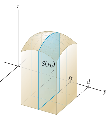
Probabilities of events: Continuous case Let be the rectangular region defined by such that and . Then:
For more general regions :
The existence of a variable does not change the theory for a variable considered by itself.
However, it is possible to relate the theory for to the theory for , in various ways.
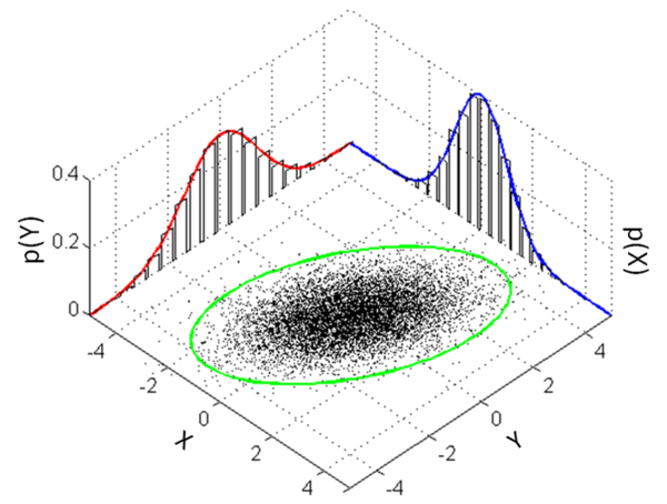
The simplest relationship is the marginal distribution for , which is merely the distribution of itself, considered as a single random variable, but in a context where it is derived from the joint distribution for .
Marginal PMF, marginal PDF
Marginal distributions are obtained from joint distributions by summing the probabilities over all possibilities of the other variable.
Discrete marginal PMF:
Continuous marginal PMF:
Infinitesimal method
Suppose has density that is continuous at . Then for infinitesimal :
Suppose and have joint density that is continuous at . Then for infinitesimal :
Joint densities depend on coordinates
The density in these integration formulas depends on the way and act as Cartesian coordinates and determine differential areas as little rectangles.
To find a density in polar coordinates, for example, it is not enough to solve for and and plug into !
Instead, we must consider the differential area vs. . We find that .
As an example, the density of the uniform distribution on the unit disk is , which is not constant as a function of and .
Link to originalExtra - Joint densities may not exist
It is not always possible to form a joint PDF from any two continuous RVs and .
For example, if , then cannot have a joint PDF, since but the integral over the region will always be 0. (The area of a line is zero.)
02 Illustration
Example - Smaller and bigger rolls
Joint and marginal PMFs - Smaller and bigger roll
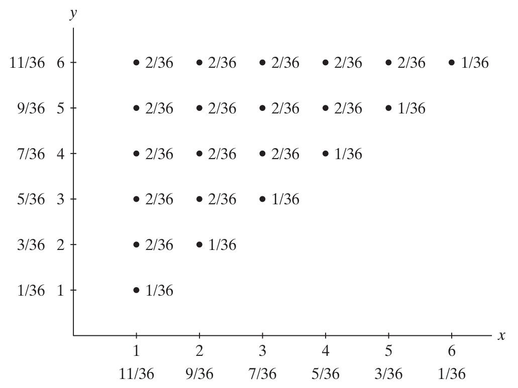
Roll two dice, and let indicate the smaller of the numbers rolled, and let indicate the bigger number.
Make a chart showing the PMF. Compute the marginal probabilities, and write them in the margins of the chart.
Solution
Link to original
Exercise - Event probabilities by reading PMF table
Event probabilities by reading PMF table
Here is a joint PMF table:
Using the table, compute the following event probabilities:
(a) (b) (c) (d)
Link to original
Exercise - Joint and marginal PMFs - Coin flipping
Joint and marginal PMFs - Coin flipping
Flip a fair coin four times. Let measure the number of heads in the first two flips, and let measure the total number of heads.
Make a chart showing the PMF. Compute the marginal probabilities, and write them in the margins of the chart.
Link to original
Example - Marginal and event probability from joint density
Marginal and event probability from joint density
Suppose the joint density of and is given by:
Find (a) and (b) .
Solution
(a)
When , the range is to :
When , the range is to :
Therefore:
(b)
Find probability of the event :
Link to original
Exercise - Marginals from joint density
Marginals from joint density
The joint PDF for and is given by:
Find and .
Link to original
Exercise - Event probability from joint density
Event probability from joint density
The joint PDF for and is given by:
Compute .
Link to original
03 Theory
Theory 2
Joint CDF
The joint CDF of and is defined by:
We can relate the joint CDF to the joint PDF using integration:
Conversely, if and have a continuous joint PDF that is also differentiable, we can obtain the PDF from the CDF using partial derivatives:
There is also a marginal CDF that is computed using a limit:
This could also be written, somewhat abusing notation, as .
Link to original
04 Illustration
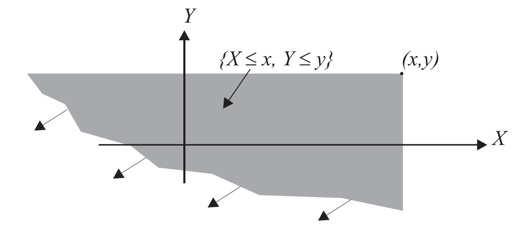
Exercise - Properties of joint CDFs
Properties of joint CDFs
(a) Show with a drawing that if both and , we know:
(b) Explain why:
(c) Explain why:
Link to original
Independent random variables
05 Theory
Theory 1
Independent random variables
Random variables are independent when they satisfy the product rule for all valid subsets :
Since , this definition is equivalent to independence of all events constructible using the variables and .
For discrete random variables, it is enough to check independence for simple events of type and for and any possible values of and .
The independence criterion for random variables can be cast entirely in terms of their distributions and written using the PMFs or PDFs.
Independence using PMF and PDF
Discrete case:
Continuous case:
Link to originalIndependence via joint CDF
Random variables and are independent when their CDFs obey the product rule:
06 Illustration
Example - Meeting in the park
Event probability - Meeting in the park
A man and a woman arrange to meet in the park between 12:00 and 1:00pm. They both arrive at a random time with uniform distribution over that hour, and do not coordinate with each other.
Find the probability that the first person to arrive has to wait longer than 15 minutes for the second person to arrive.
Solution
Let denote the time the man arrives. Use minutes starting from 12:00, so . Let denote the time the woman arrives, using the same interval.
The probability we seek is:
Because and are symmetrical in probability, these terms have the same value, so we just double the first one for our answer.
Since the arrivals are independent of each other, we have .
Since each arrival time is uniform over the interval, we have:
Therefore the joint density is . Calculate:
Link to original
Example - Uniform disk: Cartesian vs. polar
Uniform disk: Cartesian vs. polar
Suppose that a point is chosen uniformly at random on the unit disk.
(a) Let and be the Cartesian coordinates of the chosen point. Are and independent?
(b) Let and give the polar coordinates of the chosen point. Are and independent?
Solution
(a)
Write for the joint distribution of and . We have:
Then computing , we obtain:
By similar reasoning, for .
The product is not equal to , so and are not independent. Information about the value of does provide constraints on the possible values of , so this result makes sense.
(b)
To find the marginals and , the standard method is to integrate the density in the opposite variables.
varies!
The probability density is not constant! The area of a differential sector depends on .
We can take two approaches to finding the density :
(i) Area of a differential sector divided by total area:
So the density is .
(ii) Via the CDF:
Joint PDF from joint CDF: uniform distribution in polar
The region ‘below’ a given point , in polar coordinates, is a sector with area . The factor is a percentage of the circle with area .
The density is a constant across the disk, so the CDF at is this same area times . Thus:
Then in polar coordinates the density is given by taking partial derivatives:
Once we have , integrate to get the marginals:
Check independence:
In this problem it is feasible to find the marginals directly, without computing the new density, only using some geometric reasoning.
Link to originalExtra - Infinitesimal method for the marginals
The probability is the area (over ) of a thickened circle with radius and thickness . The circumference of a circle at radius is . So the area of the thickened circle is . So the probability is . This tells us that the marginal probability density is .
The probability is the area (over ) of a thin sector with radius 1 and angle . This area is . So the probability is . This tells us that the marginal probability density is .
These results agree with those above from differentiating the CDF.