W09 Notes

Functions on two random variables

01 Theory

Theory 1

PMF of (any) function of two discrete variables

Suppose $W=g(X,Y)$ and $X,Y$ are discrete RVs.

The PMF of $W$:

$$P_W(w)=\sum _{{g(x,y)=w}^{(x,y)\text{ s.t.}}}{P}_{X,Y}(x,y)$$

CDF of (continuous) function of two continuous variables

Suppose $W=g(X,Y)$ and $X,Y$ are continuous RVs, and $g$ is a continuous function.

The CDF of $W$:

$$F_W(w)=P[W\le w]=\underset{g(x,y)\le w}{\iint }{f}_{X,Y}(x,y)dxdy$$

If desired, one can then compute the PDF of $W$ by differentiating the continuous CDF:

$$f_W(w)=\frac{d}{dw}{F}_W(w)$$Link to original

02 Illustration

Exercise - PMF of $X{Y}^2$ from chart

PMF of XY squared from chart

Suppose the joint PMF of $X$ and $Y$ is given by this chart:

$Y\downarrow X\to$	$1$	$2$
$-1$	0.2	0.2
$0$	0.35	0.1
$1$	0.05	0.1

Define $W=X{Y}^2$.

(a) Find the PMF $P_W(w)$.

(b) Find the expectation $E[W]$.

Link to original

Example - Max and Min from joint PDF

Max and Min from joint PDF

Suppose the joint PDF of $X$ and $Y$ is given by:

$$f_{X,Y}(x,y)=\{\begin{array}{cc}\frac{3}{2}(x^2+y^2)& x,y\in [\mathrm{0,1}]\\ 0& \text{otherwise}\end{array}$$

Find the PDF of (a) $W=\mathrm{Max}(X,Y)$, and of (b) $W=\mathrm{Min}(X,Y)$.

Solution

(a)

(1) Compute CDF of $W$:

Convert to event form:

$$\begin{array}{c}{F}_W(w)=P[\mathrm{Max}(X,Y)\le w]\\ \\ \gg \gg P[X\le w\text{and}Y\le w]\end{array}$$

Integrate PDF over the region, assuming $w\in [\mathrm{0,1}]$:

$$\begin{array}{c}{\int }_{-\infty }^w{\int }_{-\infty }^w{f}_{X,Y}(x,y)dxdy\\ \\ \gg \gg {\int }_0^w{\int }_0^w\frac{3}{2}(x^2+y^2)dxdy\gg \gg w^4\end{array}$$

---

(2) Differentiate to find $f_W(w)$:

$f_W=\frac{d}{dw}{F}_W(w)$:

$$f_W(w)=\{\begin{array}{cc}4w^3& w\in [\mathrm{0,1}]\\ 0& \text{otherwise}\end{array}$$

---

(b)

(1) Compute CDF of $W$:

Convert to event form:

$$\begin{array}{c}{F}_W(w)=P[\mathrm{Min}(X,Y)\le w]\\ \\ \gg \gg 1-P[\mathrm{Min}(X,Y)>w]\\ \\ \gg \gg 1-P[X>w\text{and}Y>w]\end{array}$$

Integrate PDF over the region:

$$\begin{array}{c}P[X>w\text{and}Y>w]\gg \gg {\int }_w^1{\int }_w^1\frac{3}{2}(x^2+y^2)dxdy\\ \\ \gg \gg w^4-w^3-w+1\end{array}$$

Therefore:

$$F_W(w)=-w^4+w^3+w$$

---

(2) Differentiate to find $f_W(w)$:

$f_W=\frac{d}{dw}{F}_W(w)$:

$$f_W(w)=\{\begin{array}{cc}-4w^3+3w^2+1& w\in [\mathrm{0,1}]\\ 0& \text{otherwise}\end{array}$$ Link to original

Example - PDF of a sum

PDF of sums practice

Suppose $X$ is an RV with density:

$$f_X=\{\begin{array}{cc}2x& x\in [\mathrm{0,1}]\\ 0& \text{otherwise}\end{array}$$

Suppose $Y$ is uniform on $[\mathrm{0,1}]$ and independent of $X$.

Find the PDF of $X+Y$. Sketch the graph of this PDF.

Solution

(1) Write the CDF of $W=X+Y$ as a double integral:

$$F_W(w)=P[X+Y\le w]={\iint }_{x+y\le w}{f}_{X,Y}dxdy$$

The joint density on the unit square $x\in [\mathrm{0,1}],y\in [\mathrm{0,1}]$ is:

$$f_{X,Y}\gg \gg f_X\cdot f_Y\gg \gg 2x\cdot 1\gg \gg 2x$$

There is positive density in the region $x+y\le w$ only for $x\le w$ (otherwise $y<0$).

• When $w\in [\mathrm{0,1}]$, there is positive density in the region (only) when $y\le w-x$.
• When $w\in [\mathrm{1,2}]$, there is positive density in the region whenever $y\le 1$.

---

(2) Evaluate $F_W(w)$ for $w\in [\mathrm{0,1}]$:

Here $x\in [0,w]$ and $w-x\le 1$, so $y\in [0,w-x]$.

$$\begin{array}{c}{F}_W(w)={\int }_0^w{\int }_0^{w-x}2xdydx\\ \\ \gg \gg {\int }_0^{w}2x(w-x)dx\gg \gg {[w{x}^2-\frac{2x^3}{3}]}_0^w\\ \\ \gg \gg w^3-\frac{2w^3}{3}\gg \gg \frac{w^3}{3}\end{array}$$

Differentiate:

$$f_W(w)=\frac{d}{dw}\frac{w^3}{3}\gg \gg w^2$$

---

(3) Evaluate $F_W(w)$ for $w\in [\mathrm{1,2}]$:

Now $x$ ranges over $[\mathrm{0,1}]$. Split by whether the $y$-bound is $1$ or $w-x$:

• $x\in [0,w-1]$: $w-x\ge 1$, so $y\in [\mathrm{0,1}]$
• $x\in [w-1,1]$: $w-x<1$, so $y\in [0,w-x]$

$$\begin{array}{c}{F}_W(w)={\int }_0^{w-1}{\int }_0^{1}2xdydx+{\int }_{w-1}^1{\int }_0^{w-x}2xdydx\\ \\ \gg \gg {\int }_0^{w-1}2xdx+{\int }_{w-1}^{1}2x(w-x)dx\\ \\ \gg \gg (w-1{)}^2+{[w{x}^2-\frac{2x^3}{3}]}_{w-1}^1\\ \\ \gg \gg (w-1{)}^2+(w-\frac{2}{3})-(w(w-1{)}^2-\frac{2(w-1{)}^3}{3})\\ \\ \gg \gg -\frac{1}{3}{x}^3+w^2-\frac{1}{3}\end{array}$$

---

(4) Differentiate for the final PDF:

$$f_W(w)=\frac{d}{dw}(-\frac{1}{3}{x}^3+w^2-\frac{1}{3})\gg \gg -w^2+2w$$

Therefore:

$$f_{X+Y}(w)=\{\begin{array}{cc}{w}^2& w\in [\mathrm{0,1}]\\ & \\ -w^2+2w& w\in [\mathrm{1,2}]\\ & \\ 0& \text{otherwise}\end{array}$$ Link to original

Extra - Convolution

Convolution

Extra Example - PDF of a quotient

PDF of a quotient

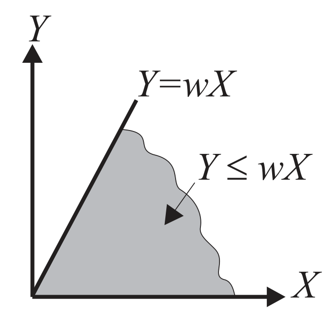
Suppose the joint PDF of $X$ and $Y$ is given by:

$$f_{X,Y}(x,y)=\{\begin{array}{cc}\lambda \mu e^{-(\lambda x+\mu y)}& x,y\ge 0\\ 0& \text{otherwise}\end{array}$$

Find the PDF of $W=g(X,Y)$ for $g(X,Y)=Y/X$.

Solution

(1) Find the CDF using logic:

$$\begin{array}{c}{F}_W(w)=P[Y/X\le w]\\ \\ \gg \gg P[Y\le wX]\end{array}$$

Integrate over this region:

$$\begin{array}{cc}P[Y\le wX]& ={\int }_0^{\infty }{\int }_0^{wx}{f}_{X,Y}(x,y)dydx\\ & \\ & \gg \gg {\int }_0^{\infty }\lambda e^{-\lambda x}{\int }_0^{wx}\mu e^{-\mu y}dydx\\ & \\ & \gg \gg {\int }_0^{\infty }\lambda e^{-\lambda x}(-e^{-\mu wx}+1)dx\\ & \\ & \gg \gg 1-\frac{\lambda }{\lambda +\mu w}\end{array}$$

---

(2) Differentiate to find PDF:

Compute $\frac{d}{dw}{F}_W(w)$:

$$f_W(w)=\{\begin{array}{cc}{\displaystyle \frac{\lambda \mu }{{(\lambda +\mu w)}^2}}& w\ge 0\\ & \\ 0& \text{otherwise}\end{array}$$Link to original

03 Theory

Theory 6

Recall that in a Poisson process:

• $X\sim \mathrm{Exp}(\lambda )$ measures continuous wait time until one arrival
• $X\sim \mathrm{Erlang}(\ell ,\lambda )$ measures continuous wait time until ${\ell }^{\text{th}}$ arrival

Since the wait times between arrivals are independent, we expect that the sum of exponential distributions is an Erlang distribution. This is true!

Erlang sum rule

Specify a given Poisson process with arrival rate $\lambda$. Suppose that:

• $X\sim \mathrm{Erlang}(r,\lambda )$ for any $r=1,2,3,\dots$
• $Y\sim \mathrm{Erlang}(s,\lambda )$ or any $s=1,2,3,\dots$
• $X$ and $Y$ are independent

Then:

$$X+Y\sim \mathrm{Erlang}(r+s,\lambda )$$

Exp plus Exp is Erlang

Recall that $\mathrm{Erlang}(1,\lambda )\sim \mathrm{Exp}(\lambda )$.

So we could say: $\text{“}\mathrm{Exp}(\lambda )+\mathrm{Exp}(\lambda )\sim \mathrm{Erlang}(2,\lambda )\text{”}$

And:

$$\text{“}\mathrm{Exp}(\lambda )+\mathrm{Erlang}(\ell ,\lambda )\sim \mathrm{Erlang}(\ell +1,\lambda )\text{”}$$

Link to original

04 Illustration

Example - Exp plus Exp equals Erlang

Exp plus Exp equals Erlang - Without Convolution

Let us verify this formula by direct calculation:

$$\text{“}\mathrm{Exp}(\lambda )+\mathrm{Exp}(\lambda )\sim \mathrm{Erlang}(2,\lambda )\text{”}$$

Solution

Let $X,Y\sim \mathrm{Exp}(\lambda )$ be independent RVs, and let $W=X+Y$.

Therefore:

$$f_{X,Y}(x,y)=\lambda e^{-\lambda x}\cdot \lambda e^{-\lambda y}={\lambda }^2{e}^{-\lambda (x+y)}x\ge 0,y\ge 0$$

---

(1) Write the CDF as a double integral over the region $x\ge 0,y\ge 0,x+y\le w$:

For $w\ge 0$, the region is $x\in [0,w]$, $y\in [0,w-x]$.

$$F_W(w)={\int }_0^w{\int }_0^{w-x}{\lambda }^2{e}^{-\lambda (x+y)}dydx$$

---

(2) Evaluate the inner integral:

$$\begin{array}{c}{\int }_0^{w-x}{\lambda }^2{e}^{-\lambda x}{e}^{-\lambda y}dy\gg \gg {\lambda }^2{e}^{-\lambda x}{[-\frac{1}{\lambda }{e}^{-\lambda y}]}_0^{w-x}\\ \\ \gg \gg \lambda e^{-\lambda x}(1-e^{-\lambda (w-x)})\\ \\ \gg \gg \lambda (e^{-\lambda x}-e^{-\lambda w})\end{array}$$

---

(3) Evaluate the outer integral:

$$\begin{array}{c}{F}_W(w)=\lambda {\int }_0^w(e^{-\lambda x}-e^{-\lambda w})dx\\ \\ \gg \gg \lambda {[-\frac{1}{\lambda }{e}^{-\lambda x}-x{e}^{-\lambda w}]}_0^w\\ \\ \gg \gg \lambda [(-\frac{1}{\lambda }{e}^{-\lambda w}-w{e}^{-\lambda w})-(-\frac{1}{\lambda })]\\ \\ \gg \gg 1-e^{-\lambda w}-\lambda w{e}^{-\lambda w}\end{array}$$

---

(4) Differentiate for the PDF:

$$\begin{array}{c}{f}_W(w)=\frac{d}{dw}(1-e^{-\lambda w}-\lambda w{e}^{-\lambda w})\\ \\ \gg \gg \lambda e^{-\lambda w}-\lambda e^{-\lambda w}+{\lambda }^{2}w{e}^{-\lambda w}\\ \\ \gg \gg {\lambda }^{2}w{e}^{-\lambda w}\end{array}$$

This is the $\mathrm{Erlang}(2,\lambda )$ density function:

$${\frac{{\lambda }^{\ell }}{(\ell -1)!}{t}^{\ell -1}{e}^{-\lambda t}|}_{\ell =2}$$ Link to original

Exercise - Erlang induction step

Erlang induction step

Derive the formula:

$$\text{“}\mathrm{Exp}(\lambda )+\mathrm{Erlang}(\ell ,\lambda )\sim \mathrm{Erlang}(\ell +1,\lambda )\text{”}$$

Observation: By repeatedly applying the above formula, we see that:

$$\text{“}\stackrel{\ell \text{ terms}}{\overbrace{\mathrm{Exp}(\lambda )+\cdots +\mathrm{Exp}(\lambda )}}\sim \mathrm{Erlang}(\ell ,\lambda )\text{”}$$Link to original