Repeated trials
01 Theory
Theory 1
Repeated trials
When a single experiment type is repeated many times, and we assume each instance is independent of the others, we say it is a sequence of repeated trials or independent trials.
The probability of any sequence of outcomes is derived using independence together with the probabilities of outcomes of each trial.
A simple type of trial, called a Bernoulli trial, has two possible outcomes, 1 and 0, or success and failure, or and . A sequence of repeated Bernoulli trials is called a Bernoulli process.
- Write sequences like for the outcomes of repeated trials of this type.
- Independence implies
- Write and , and because these are all outcomes (exclusive and exhaustive), we have . Then:
- This gives a formula for the probability of any sequence of these trials.
A more complex trial may have three outcomes, , , and .
- Write sequences like for the outcomes.
- Label and and . We must have .
- Independence implies
- This gives a formula for the probability of any sequence of these trials.
Let stand for the sum of successes in some Bernoulli process. So, for example, “” stands for the event that the number of successes is exactly 3. The probabilities of events follow a binomial distribution.
Suppose a coin is biased with , and is ‘success’. Flip the coin 20 times. Then:
Each outcome with exactly 3 heads and 17 tails has probability . The number of such outcomes is the number of ways to choose 3 of the flips to be heads out of the 20 total flips.
The probability of at least 18 heads would then be:
With three possible outcomes, , , and , we can write sum variables like which counts the number of outcomes, and and similarly. The probabilities of events like follow a multinomial distribution.
Link to original
02 Illustration
Example - Multinomial: Soft drinks preferred
Multinomial: Soft drinks preferred
Folks coming to a party prefer Coke (55%), Pepsi (25%), or Dew (20%). If 20 people order drinks in sequence, what is the probability that exactly 12 have Coke and 5 have Pepsi and 3 have Dew?
Solution
The multinomial coefficient gives the number of ways to assign 20 people into bins according to preferences matching the given numbers, and and .
Each such assignment is one sequence of outcomes. All such sequences have probability .
The answer is therefore:
Link to original
Reliability
03 Theory
Theory 1
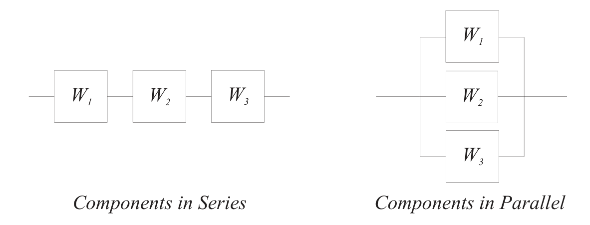
Consider some process schematically with components in series and components in parallel:
- Each component has a probability of success or failure.
- Event indicates ‘success’ of that component (same name).
- Then is the probability of succeeding.
Success for a series of components requires success of each member.
- Series components rely on each other.
- Success of the whole is success of part 1 AND success of part 2 AND part 3, etc.
Failure for parallel components requires failure of each member.
- Parallel components represent redundancy.
- Success of the whole is success of part 1 OR success of part 2 OR part 3, etc.
For series components, stack successes:
For parallel components, stack failures:
E.g. if for all components , then:
- Series components:
- Parallel components:
To analyze a complex diagram of series and parallel components, bundle each:
- pure series set as a single compound component with its own success probability (the product)
- pure parallel set as a single compound component with its own success probability (using the failure formula)
This is like the analysis of resistors and inductors.
Link to original
04 Illustration
Example - Series, parallel, series
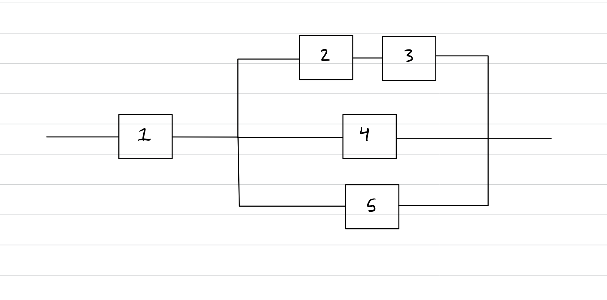
Reliability: Series, parallel, series
Suppose a process has internal components arranged like this:
Write for the event that component succeeds, and for the event that it fails.
The success probabilities for each component are given in the chart:
1 2 3 4 5 92% 89% 95% 86% 91% Find the probability that the entire system succeeds.
Solution
For intersections, use (independence) and for unions, use .
So and:
Link to original
Random variables
05 Theory
Theory 1
Random variable
A random variable (RV) on a probability space is a function .
So assigns to each outcome a number.
Note: The word ‘variable’ indicates that an RV outputs numbers.
Random variables can be formed from other random variables using mathematical operations on the output numbers.
Given random variables and , we can form these new ones:
Suppose is some particular outcome. Then, for example, is by definition .
Random variables determine events.
- Given , the event “” is equal to the set
- That is: the set of outcomes mapped to by
- That is: the event “ took the value ”
Such events have probabilities. We write them like this:
This generalized to events where lies in some range or set, for example:
The axioms of probability translate into rules for these events.
For example, additivity leads to:
A discrete random variable has probability concentrated at a discrete set of real numbers.
- A ‘discrete set’ means finite or countably infinite.
- The distribution of probability is recorded using a probability mass function (PMF) that assigns probabilities to each of the discrete real numbers.
- Numbers with nonzero probability are called possible values.
PMF
The PMF function , for a discrete RV, is defined by:
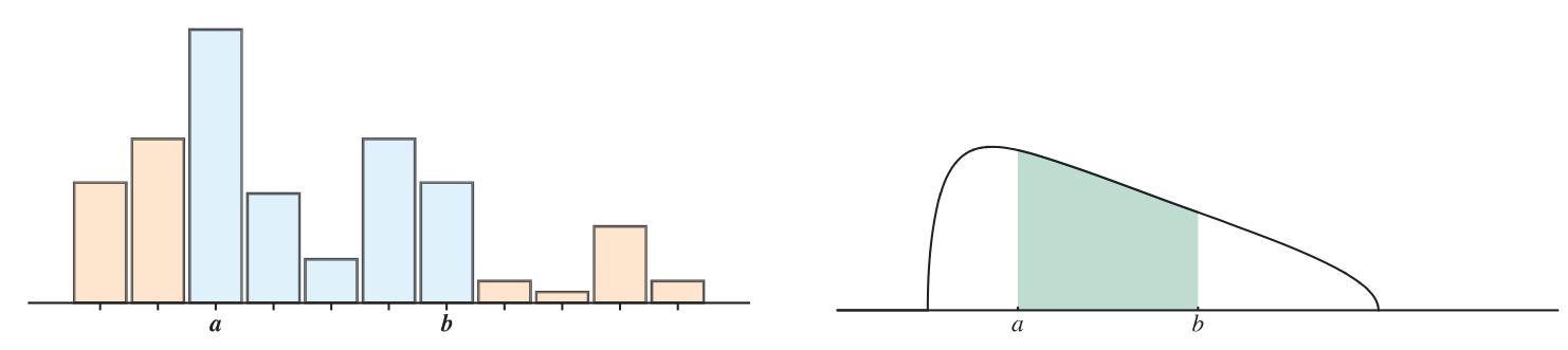
A continuous random variable has probability spread out over the space of real numbers.
- The distribution of probability is recorded using a probability density function (PDF) which is integrated over intervals to determine probabilities.
The PDF function for (a CRV) is written for , and probabilities are calculated like this:
For any RV, whether discrete or continuous, the distribution of probability is encoded by a function:
CDF
The cumulative distribution function (CDF) for a random variable is defined for all by:
Notes:
- Sometimes the relation to is omitted and one sees just “.”
- Sometimes the CDF is called, simply, “the distribution function” because:
The CDF works for a discrete, continuous, or mixed RV
- PMF is for discrete only
- PDF is for continuous only
- CDF covers both and covers mixed RVs
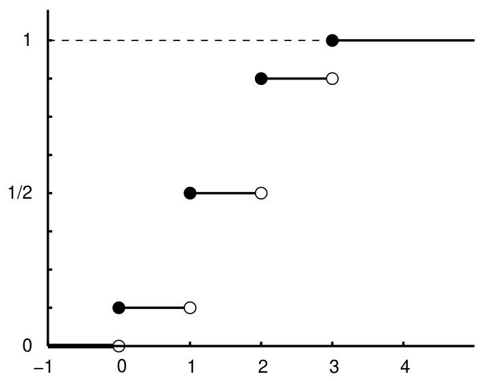
The CDF of a discrete RV is always a stepwise increasing function. At each step up, the jump size matches the PMF value there.
From this graph of :
we can infer the PMF values based on the jump sizes:
For a discrete RV, the CDF and the PMF can be calculated from each other using formulas.
Link to originalPMF from CDF
Given a PMF , the CDF is determined by:
where is the set of possible values of .
06 Illustration
Example - PDF and CDF: Roll 2 dice
PDF and CDF: Roll 2 dice
Roll two dice colored red and green. Let record the number of dots showing on the red die, the number on the green die, and let be a random variable giving the total number of dots showing after the roll, namely .
- Find the PMFs of and of and of .
- Find the CDF of .
- Find .
Solution
(1) Construct sample space:
Denote outcomes with ordered pairs of numbers , where is the number showing on the red die and is the number on the green one.
Therefore are integers satisfying .
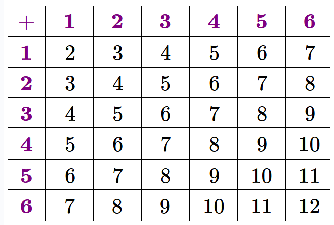
(2) Create chart of outcomes:
(3) Define random variables:
We have and .
Therefore .
(4) Find PMF of :
Use variable for each possible value of , so . Find :
Therefore for every .
(5) Find PMF of similarly:
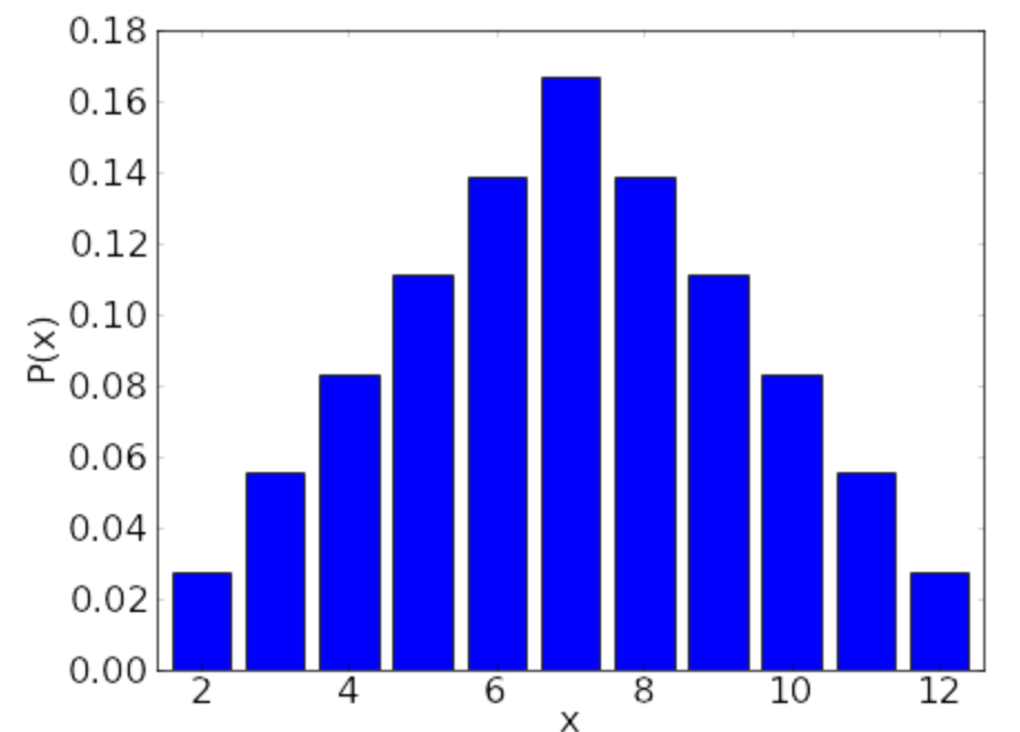
(6) Find PMF of :
Count outcomes along diagonal lines in the chart.
2 3 4 5 6 7 8 9 10 11 12
Evaluate: .
(7) Find CDF of :
CDF definition:
Apply definition: add new PMF value at each increment:
Link to original
Example - Total heads count; binomial expansion of 1
PMF for total heads count; binomial expansion of 1
A fair coin is flipped times.
Let be the random variable that counts the total number of heads in each sequence.
The PMF of is given by:
Since the total probability must add to 1, we know this formula must hold:
Is this equation really true?
There is another way to view this equation: it is the binomial expansion where and :
Link to original
Example - Life insurance payouts
Life insurance payouts
A life insurance company has two clients, and , each with a policy that pays $100,000 upon death. Consider events that the older client dies next year, and that the younger dies next year. Suppose and .
Define a random variable measuring the total money paid out next year in units of $1,000. The possible values for are 0, 100, 200. Now calculate:
Link to original
Example - Probabilities via CDF
Probabilities via CDF
Suppose the CDF of is given by . Compute:
(a) (b) (c) (d)
Link to originalSolution
(a)
(b) Same as (a) because (single point in a continuous distribution).
(c)
(d)