More polar curves
01 Theory - Polar limaçons
Theory 2
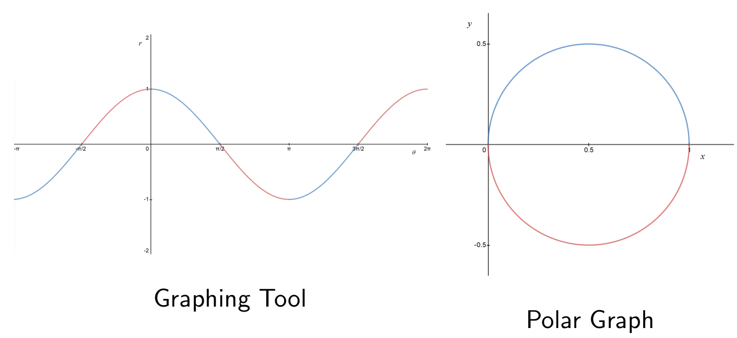
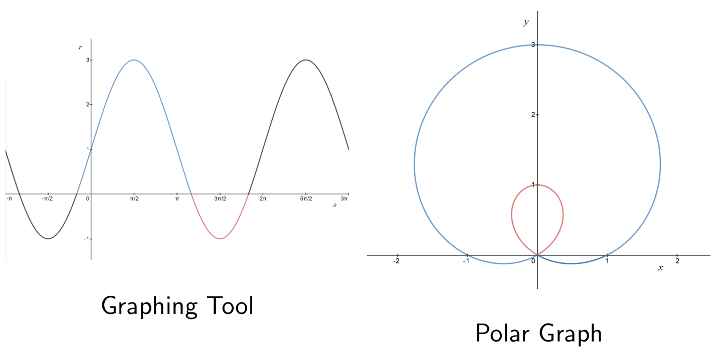
To draw the polar graph of some function, it can help to first draw the Cartesian graph of the function. (In other words, set and , and draw the usual graph.) By tracing through the points on the Cartesian graph, one can visualize the trajectory of the polar graph.
This Cartesian graph may be called a graphing tool for the polar graph.
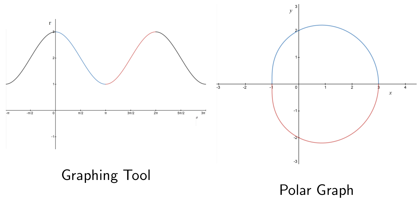
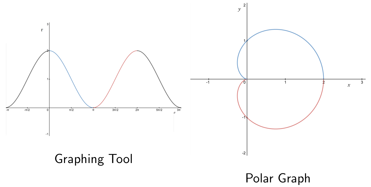
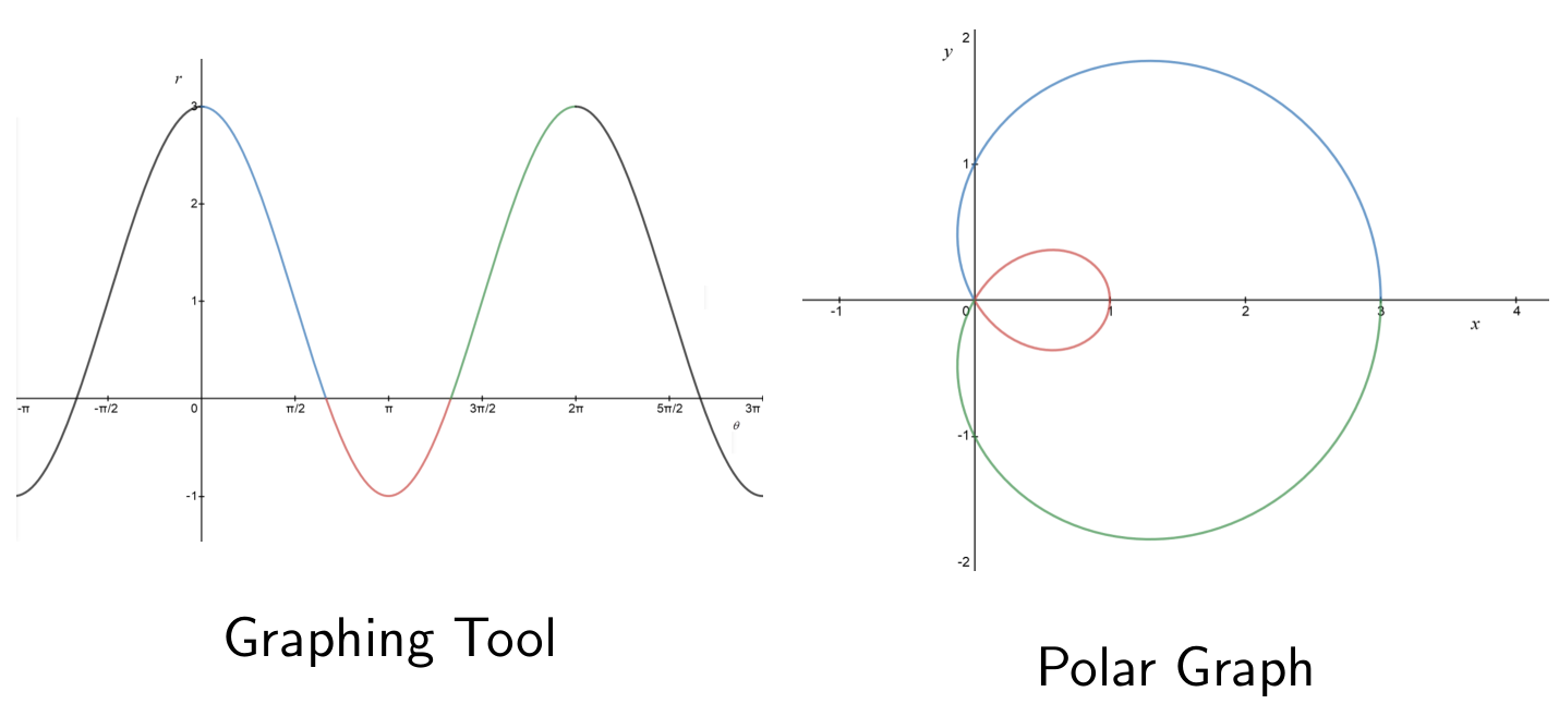
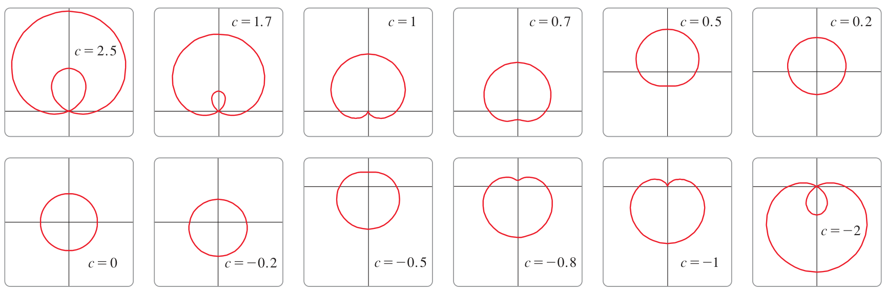
A limaçon is the polar graph of .
The shape of a limaçon is determined by the value of . Any limaçon can be rescaled to have this form:
: Limaçon satisfying : unit circle.
: Limaçon satisfying : ‘outer loop’ circle with ‘flat spot’, not quite a ‘dimple’:
: Limaçon satisfying : ‘cardioid’ ‘outer loop’ circle with ‘dimple’ that creates a cusp:
: Limaçon satisfying : ‘dimple’ pushes past cusp to create ‘inner loop’:
: Limaçon satisfying : ‘inner loop’ only, no outer loop exists:
: Limaçon satisfying : ‘inner loop’ and ‘outer loop’ and rotated :
Transitions between limaçon types, :
Notice the transition points at and :
The flat spot occurs when
- Smaller gives convex shape
The cusp occurs when
Link to original
- Smaller gives dimple (assuming )
- Larger gives inner loop
02 Theory - Polar roses
Theory 3
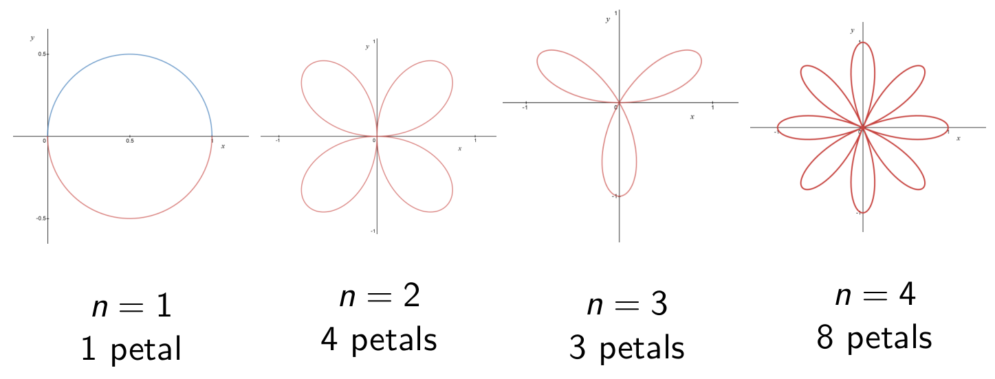
Roses are polar graphs of this form:
The pattern of petals:
Link to original
- (even): obtain petals
- These petals traversed once
- (odd): obtain petals
- These petals traversed twice
- Either way: total-petal-traversals: always
03 Illustration
Example - Finding vertical tangents to a limaçon
Finding vertical tangents to a limaçon
Let us find the vertical tangents to the limaçon (the cardioid) given by .
Solution
(1) Convert to Cartesian parametric using and :
(2) Compute and :
(3) The vertical tangents occur when . We must double check that at these points.
Substitute and observe quadratic:
Solve:
Then find :
(4) Compute the points. In polar coordinates:
In Cartesian coordinates:
At :
At :
At :
(5) Correction: is a cusp!
The point at is on the cardioid, but the curve is not smooth there, this is a cusp.
Still, the left- and right-sided tangents exists and are equal, so in a certain sense we could say the curve has vertical tangent at .
Link to original
Calculus with polar curves
04 Theory - Polar tangent lines, arclength
Theory 1
Polar arclength formula
The arclength of the polar graph of , for :
To derive this formula, convert to Cartesian with parameter :
From here you can apply the familiar arclength formula with in the place of .
Link to originalExtra - Derivation of polar arclength formula
Let and convert to parametric Cartesian, so:
Then:
Therefore:
Therefore:
05 Illustration
Example - Length of the inner loop
Length of the inner loop
Consider the limaçon given by .
How long is the inner loop? Set up an integral for this quantity.
Solution
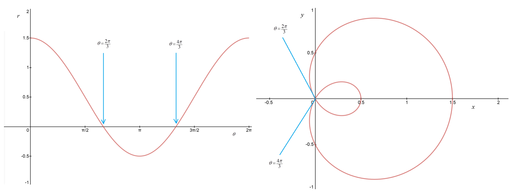
The inner loop is traced by the moving point when . This can be seen from the graph:
Therefore the length of the inner loop is given by this integral:
Link to original
06 Theory - Polar area
Theory 2
Sectorial area from polar curve
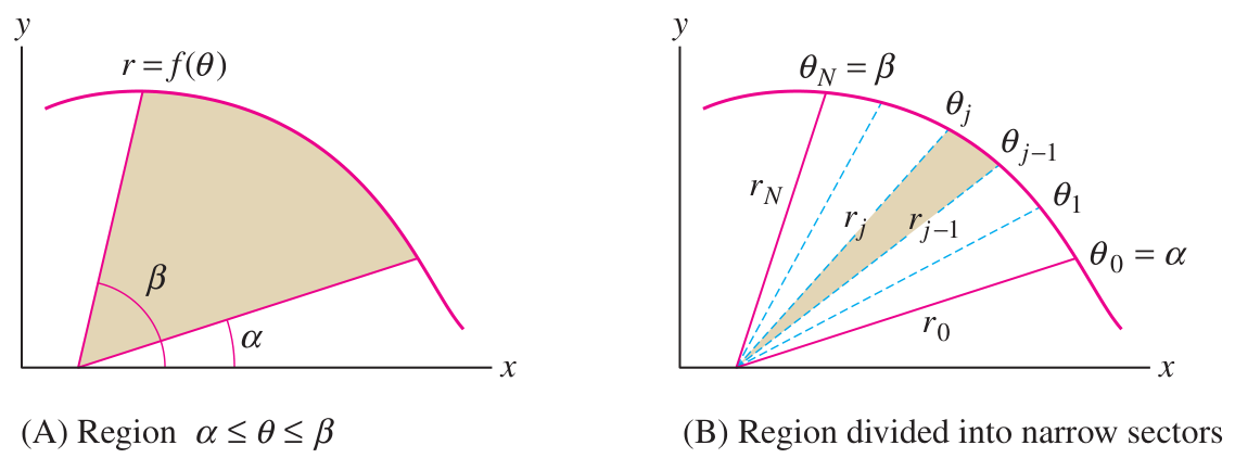
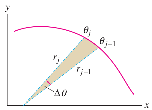
The “area under the curve” concept for graphs of functions in Cartesian coordinates translates to a “sectorial area” concept for polar graphs. To compute this area using an integral, we divide the region into Riemann sums of small sector slices.
To obtain a formula for the whole area, we need a formula for the area of each sector slice.
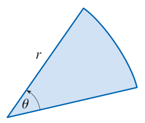
Area of sector slice
Let us verify that the area of a sector slice is .
Take the angle in radians and divide by to get the fraction of the whole disk.
Then multiply this fraction by (whole disk area) to get the area of the sector slice.
Now use and for an infinitesimal sector slice, and integrate these to get the total area formula:
One easily verifies this formula for a circle.
Let be a constant. Then:
The sectorial area between curves:
Sectorial area between polar curves
Link to originalSubtract after squaring, not before!
This aspect is not similar to the Cartesian version:
07 Illustration
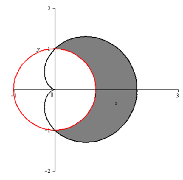
Area between circle and limaçon
Area between circle and limaçon
Find the area of the region enclosed between the circle and the limaçon .
Solution
First draw the region:
The two curves intersect at . Therefore the area enclosed is given by integrating over :
Link to original
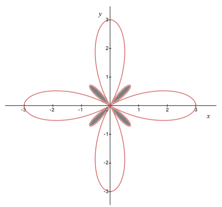
Area of small loops
Area of small loops
Consider the following polar graph of :
Find the area of the shaded region.
Solution
Find bounds for one small loop. Lower left loop occurs first. This loop is when .
Now set up area integral:
Power-to-frequency conversion: with :
Link to original
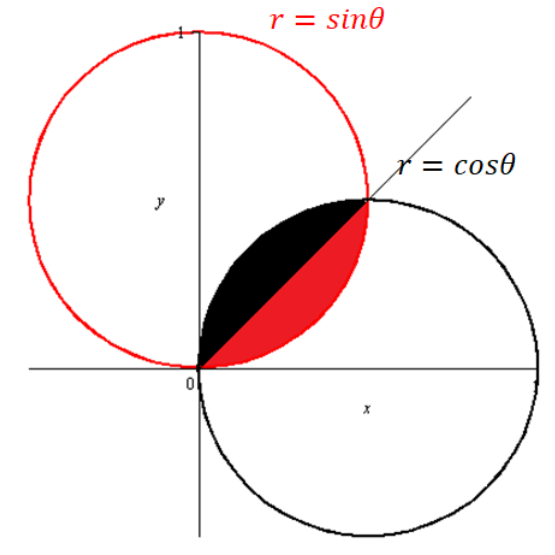
Overlap area of circles
Overlap area of circles
Compute the area of the overlap between crossing circles. For concreteness, suppose one of the circles is given by and the other is given by .
Solution
Drawing of the overlap:
Notice: total overlap area = area of red region. Bounds for red region: .
Area formula applied to :
Power-to-frequency: :
Link to original